
Every financial decision involves uncertainty. Whether choosing between investment opportunities, evaluating insurance policies, or assessing business ventures, the ability to quantify potential outcomes separates informed decisions from pure guesswork.
Expected value is the mathematical foundation for rational decision-making under uncertainty. This concept calculates the long-term average outcome of a decision by weighing each possible result by its probability of occurring. Understanding expected value transforms how investors evaluate risk, assess opportunities, and build wealth through data-driven insights rather than emotion or speculation.
The math behind money becomes clearer when expected value principles guide investment choices. This comprehensive guide explains what expected value means, how to calculate it using a simple formula, and how to apply it to real investing decisions that impact wealth building.
Key Takeaways
Expected value calculates the long-term average outcome by multiplying each possible result by its probability and summing all possibilities
Positive expected value doesn’t guarantee profit in the short term due to variance, but it favors success over many repeated decisions
Investors use expected value to compare opportunities, assess risk-adjusted returns, and avoid negative-EV decisions like gambling
Expected value differs from simple averages because it weights outcomes by their likelihood, not treating all scenarios equally
Understanding expected value prevents common mistakes like confusing probability with certainty or ignoring the size of potential losses
What Is Expected Value? (Simple Definition)
Expected value represents the average outcome anticipated from a decision if repeated many times under identical conditions. Think of it as the long-term mean result weighted by probability.
In plain English: Expected value answers the question “What should I expect on average if I make this decision repeatedly?”
Consider flipping a coin for money. If heads pays $2 and tails pays nothing, the expected value isn’t $2 or $0—it’s $1. Over many flips, results average toward this middle value because each outcome occurs roughly half the time.
This concept applies far beyond simple games. Investors use expected value to evaluate stock positions, business owners use it to assess expansion opportunities, and insurance companies use it to price policies. The underlying principle remains constant: multiply each possible outcome by its probability, then sum the results.
Expected value provides a rational framework for comparing options when certainty doesn’t exist. It transforms subjective feelings about risk into objective numbers that enable comparison and analysis.
Why Expected Value Matters for Money Decisions
Financial decisions rarely offer guaranteed outcomes. Stock prices fluctuate, businesses succeed or fail, and economic conditions change unpredictably. Expected value provides structure to this uncertainty.
Three reasons expected value matters for investing:
- Quantifies opportunity cost — Comparing expected values reveals which option offers superior long-term returns
- Exposes hidden risks — Calculations force explicit consideration of downside scenarios and their probabilities
- Removes emotional bias — Mathematical analysis replaces fear and greed with evidence-based evaluation
Successful investors don’t chase certainty—they seek favorable expected value. Diversification strategies work precisely because they improve portfolio expected value while reducing variance.
Expected Value Formula (With Explanation)
The Expected Value Formula
The mathematical expression for expected value follows a straightforward pattern:
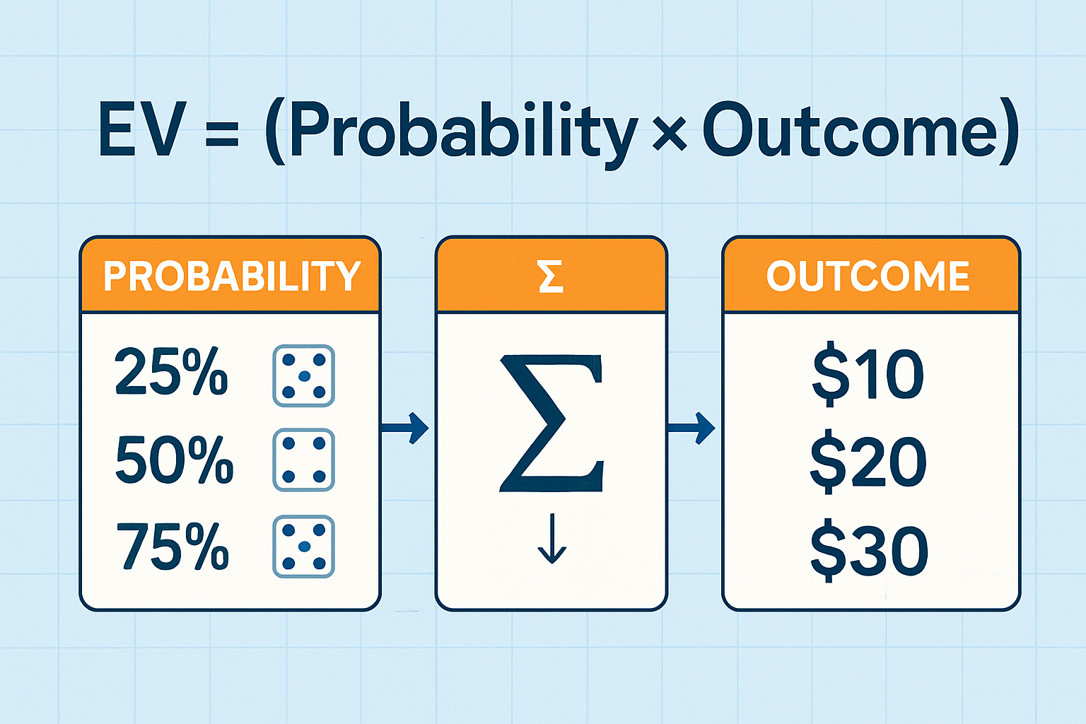
EV = Σ (Probability × Outcome)
Where:
- EV = Expected Value
- Σ = Sum of all possibilities (sigma notation)
- Probability = Likelihood of each outcome (as a decimal between 0 and 1)
- Outcome = The numerical result of each scenario
In expanded form for multiple outcomes:
EV = (P₁ × O₁) + (P₂ × O₂) + (P₃ × O₃) + … + (Pₙ × Oₙ)
This formula applies universally whether evaluating dice rolls, stock investments, or business decisions.
Breaking Down Each Component
Outcomes represent the possible results of a decision, expressed numerically. For financial applications, outcomes typically measure profit, loss, or return in dollar terms or percentages.
Example outcomes for a stock investment:
- Scenario 1: +20% return
- Scenario 2: 0% return (break-even)
- Scenario 3: -10% return (loss)
Probabilities quantify the likelihood of each outcome occurring. These values range from 0 (impossible) to 1 (certain), expressed as decimals or percentages.
Example probabilities for the stock scenarios:
- Scenario 1: 0.40 (40% chance)
- Scenario 2: 0.35 (35% chance)
- Scenario 3: 0.25 (25% chance)
Critical rule: All probabilities must sum to 1.00 (or 100%). This ensures the model accounts for all possible outcomes. If probabilities don’t total 1, the calculation contains errors or missing scenarios.
The multiplication step weights each outcome by its likelihood. High-probability outcomes influence expected value more than low-probability scenarios, even if the rare scenario offers larger payoffs.
Expected Value Examples (Step-by-Step)
Example 1: Coin Flip Bet
A friend offers a simple bet: flip a fair coin. If it lands heads, you win $10. If tails, you win nothing. What’s the expected value?
Step 1: Identify outcomes
- Heads: Win $10
- Tails: Win $0
Step 2: Determine probabilities
- Heads: 0.50 (50%)
- Tails: 0.50 (50%)
Step 3: Apply the formula
| Outcome | Probability | Value | Calculation |
|---|---|---|---|
| Heads | 0.50 | $10 | 0.50 × $10 = $5 |
| Tails | 0.50 | $0 | 0.50 × $0 = $0 |
| Total EV | $5 |
EV = (0.50 × $10) + (0.50 × $0) = $5
The expected value equals $5 per flip. Over many flips, average winnings converge toward $5 per game, even though no single flip produces exactly $5.
Example 2: Rolling a Six-Sided Die
You pay $2 to roll a standard die. You win the dollar amount shown on the die face. Should you play?
Step 1: Identify all outcomes
- Roll 1: Win $1
- Roll 2: Win $2
- Roll 3: Win $3
- Roll 4: Win $4
- Roll 5: Win $5
- Roll 6: Win $6
Step 2: Determine probabilities
Each face has equal probability: 1/6 ≈ 0.1667
Step 3: Calculate expected value
| Roll | Probability | Winnings | Calculation |
|---|---|---|---|
| 1 | 0.1667 | $1 | 0.1667 × $1 = $0.17 |
| 2 | 0.1667 | $2 | 0.1667 × $2 = $0.33 |
| 3 | 0.1667 | $3 | 0.1667 × $3 = $0.50 |
| 4 | 0.1667 | $4 | 0.1667 × $4 = $0.67 |
| 5 | 0.1667 | $5 | 0.1667 × $5 = $0.83 |
| 6 | 0.1667 | $6 | 0.1667 × $6 = $1.00 |
| Total | $3.50 |
EV = $3.50 per roll
Since the game costs $2 to play and offers $3.50 expected value, the net expected value equals $1.50 profit per roll ($3.50 – $2.00).
This represents a positive expected value opportunity. Over many plays, participants should expect to profit approximately $1.50 per game on average.
Example 3: Stock Investment Decision
An investor analyzes a stock position and estimates three possible one-year outcomes:
- Bull scenario: 30% return (probability: 30%)
- Neutral scenario: 5% return (probability: 50%)
- Bear scenario: -15% return (probability: 20%)
Calculate expected return:
| Scenario | Probability | Return | Calculation |
|---|---|---|---|
| Bull | 0.30 | +30% | 0.30 × 30% = 9.0% |
| Neutral | 0.50 | +5% | 0.50 × 5% = 2.5% |
| Bear | 0.20 | -15% | 0.20 × (-15%) = -3.0% |
| Expected Return | 8.5% |
EV = (0.30 × 30%) + (0.50 × 5%) + (0.20 × -15%) = 8.5%
The expected return equals 8.5% annually. This doesn’t guarantee an 8.5% return—actual results will match one of the three scenarios. However, the calculation suggests this investment offers positive expected value if the probability estimates prove accurate.
Comparing this 8.5% expected return against alternatives helps investors allocate capital rationally. Understanding absolute return metrics complements expected value analysis for comprehensive investment evaluation.
Key Insight: Expected Value ≠ Most Likely Outcome
Notice in the dice example that the expected value ($3.50) cannot actually occur on any single roll. The most likely outcome is any number from 1 to 6, each equally probable.
Expected value represents the long-term average, not the most probable single result.
This distinction matters enormously for investing. A stock might most likely return 5%, but if small probabilities exist for extreme gains or losses, the expected value differs significantly from the modal outcome.
Short-term results vary widely around the expected value. Only through repeated decisions or extended time periods do actual results converge toward the mathematical expectation. This principle explains why dividend investing strategies emphasize consistency and repetition over time.
Expected Value vs Average (Common Confusion)
Many beginners confuse expected value with simple averages. While related, these concepts differ in crucial ways.
Simple Average (Mean)
A simple average adds all values and divides by the count:
Average = (Sum of all values) ÷ (Number of values)
Example: The average of 2, 4, and 6 equals (2+4+6) ÷ 3 = 4
Simple averages treat all values equally, regardless of how likely each value is to occur.
Expected Value (Probability-Weighted Average)
Expected value weights each outcome by its probability before averaging:
EV = Σ (Probability × Outcome)
Expected value recognizes that not all outcomes occur with equal frequency.
When They Differ (And Why It Matters)
Consider two investment options:
Investment A outcomes: 5%, 10%, 15% (each equally likely)
- Simple average: (5% + 10% + 15%) ÷ 3 = 10%
- Expected value: (0.333 × 5%) + (0.333 × 10%) + (0.333 × 15%) = 10%
When probabilities are equal, the simple average equals the expected value.
Investment B outcomes:
- 5% return (70% probability)
- 10% return (20% probability)
- 50% return (10% probability)
- Simple average: (5% + 10% + 50%) ÷ 3 = 21.7%
- Expected value: (0.70 × 5%) + (0.20 × 10%) + (0.10 × 50%) = 10.5%
When probabilities differ, expected value provides the accurate long-term average. The simple average misleadingly suggests 21.7% returns because it weights the rare 50% outcome equally with the common 5% outcome.
For financial decisions, use expected value, not simple averages. Market returns don’t occur with equal probability—bull markets, bear markets, and neutral periods have different frequencies. Expected value calculations account for this reality.
Understanding this distinction improves analysis of annualized returns and performance metrics across different time periods.
Expected Value in Finance and Investing
Expected Value in Stock Investing
Professional investors implicitly or explicitly calculate expected value for every position. The process requires estimating potential returns and their probabilities based on fundamental analysis, market conditions, and economic factors.
Framework for stock expected value:
- Define scenarios (typically 3-5 outcomes covering the probability spectrum)
- Estimate returns for each scenario based on valuation, growth, and market factors
- Assign probabilities using historical data, analyst consensus, or subjective judgment
- Calculate expected return using the formula
- Compare against alternatives, including risk-free rates and benchmark indices
Example: Analyzing a technology stock
| Scenario | Probability | 1-Year Return | Weighted Return |
|---|---|---|---|
| Strong growth | 25% | +40% | 10.0% |
| Moderate growth | 40% | +15% | 6.0% |
| Flat performance | 20% | 0% | 0.0% |
| Decline | 15% | -20% | -3.0% |
| Expected Return | 100% | 13.0% |
If this stock’s expected return (13%) exceeds the investor’s required return or alternative opportunities, it represents a favorable expected value proposition.
Critical limitation: Expected value calculations depend entirely on probability estimates. Garbage in, garbage out. Overconfident or biased probability assessments produce misleading expected values.
This explains why diversification remains essential even when individual positions show positive expected value. Diversification protects against estimation errors in probability assignments.
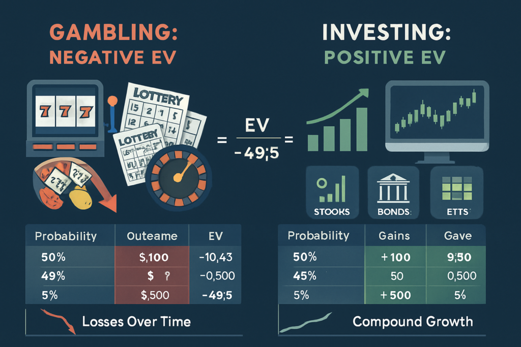
Expected Value in Gambling vs Investing
The distinction between gambling and investing often reduces to expected value analysis.
Gambling: Negative Expected Value
Casino games, lotteries, and sports betting typically feature negative expected value for participants. The house edge ensures long-term losses for players.
Lottery example:
- Ticket cost: $2
- Jackpot: $100 million
- Probability of winning: 1 in 300 million (0.00000000333)
- Expected value: 0.00000000333 × $100,000,000 = $0.33
EV = $0.33 – $2.00 cost = -$1.67 per ticket
Every lottery ticket purchased loses $1.67 on average. The occasional jackpot winner doesn’t change the mathematical reality that expected value strongly favors the lottery operator.
Investing: Positive Expected Value
Properly diversified equity investing historically delivers positive expected value. Stock markets trend upward over long periods because underlying businesses generate profits, and economic growth creates value.
S&P 500 historical analysis (1926-2024):
- Average annual return: ~10%
- Probability of positive return (any 1 year): ~73%
- Probability of positive return (any 10 years): ~94%
- Probability of positive return (any 20 years): ~100%
Long-term equity investing offers positive expected value because:
- Economic growth increases corporate earnings over time
- Dividends provide cash returns regardless of price movements
- Inflation protection preserves purchasing power better than cash
- Compound growth amplifies returns over extended periods
This fundamental difference—positive vs. negative expected value—separates wealth-building activities from wealth-destroying entertainment.
Understanding compound interest mechanics shows how positive expected value investments grow exponentially over time.
Insurance, Credit Cards, and Expected Value
Financial companies build entire business models on expected value calculations.
Insurance companies profit by charging premiums that exceed expected claim payouts:
Auto insurance example:
- Annual premium: $1,200
- Probability of claim: 5%
- Average claim payout: $15,000
- Expected payout: 0.05 × $15,000 = $750
The insurer collects $1,200 but expects to pay $750, generating $450 profit per policy on average. Across thousands of policies, this expected value gap produces reliable profits.
For policyholders, insurance represents negative expected value in pure financial terms. However, it provides value through risk transfer, exchanging small, certain losses (premiums) for protection against large, uncertain losses (accidents).
Credit card companies use expected value to price interest rates and fees:
- Interest revenue from balances
- Fee income from late payments, annual fees, etc.
- Minus: Expected default losses
- Minus: Rewards program costs
- Equals: Expected profit per customer
Companies carefully calculate expected value across their customer base, accepting that some accounts will default while others generate substantial profits. The portfolio expected value determines business viability.
Consumer application: Understanding these expected value dynamics helps evaluate whether insurance coverage or credit products offer fair value. Compare the expected value of self-insuring (saving the premium) against transferring risk to insurers.
Managing credit utilization strategically can improve the expected value of credit card relationships by maximizing rewards while avoiding interest charges.
Why Positive Expected Value Doesn’t Guarantee Profit

The most dangerous misunderstanding about expected value is assuming positive EV guarantees positive results. It doesn’t.
Variance and Volatility
Variance measures how widely actual outcomes scatter around the expected value. High variance means individual results often differ dramatically from the average.
Consider two investments with identical 10% expected returns:
Investment A: Low Variance
- 90% probability of 9% return
- 10% probability of 19% return
- Expected return: 10%
Investment B: High Variance
- 50% probability of -10% return
- 50% probability of 30% return
- Expected return: 10%
Both offer 10% expected value, but Investment B creates much greater uncertainty. Half the time, it loses money despite positive expected value.
Volatility in financial markets means even the best long-term investments experience short-term losses. The S&P 500 averages ~10% annual returns but suffers negative years roughly 27% of the time.
Positive expected value plays out over many trials or extended time periods. Individual instances or short timeframes produce highly variable results.
Short-Term Losses vs Long-Term Math
Expected value represents a long-run average, not a short-term prediction.
Flip a coin for $10 (heads) vs. $0 (tails) ten times:
- Expected value: $5 per flip
- Expected total: $50 over 10 flips
- Possible actual results: anywhere from $0 to $100
You might flip tails eight times and collect only $20 despite $50 expected value. The math doesn’t guarantee results in small samples.
Law of Large Numbers: As trials increase, actual results converge toward the expected value. With 10,000 coin flips, the results will approximate $50,000 very closely.
For investors, this principle means:
- Single positions may underperform despite positive expected value
- Short time periods (months, even years) can produce losses
- Diversification (more independent positions) accelerates convergence toward the expected value
- Long time horizons (decades) dramatically increase the probability of realizing expected returns
This explains why index fund investing over 30+ years reliably builds wealth while individual stock picks or short-term trading often disappoint.
Risk Tolerance Matters
Even with positive expected value, risk tolerance determines whether an opportunity suits an investor.
Extreme example: A bet offering 99% probability of losing $100,000 and 1% probability of winning $20 million has positive expected value:
EV = (0.99 × -$100,000) + (0.01 × $20,000,000) = $101,000
Despite a massive positive expected value, most people would decline this bet because:
- Ruin risk — The 99% loss scenario creates financial catastrophe
- Single trial — No opportunity to repeat the bet enough times for the expected value to materialize
- Utility of money — Losing $100,000 causes more harm than winning $20 million provides benefit
Kelly Criterion addresses this by calculating optimal bet sizes that maximize long-term growth while avoiding ruin risk. The formula accounts for both expected value and variance.
Smart investors seek positive expected value opportunities that also align with their risk capacity and time horizon. Expected value analysis is necessary but not sufficient for decision-making.
Understanding personal risk management needs helps balance expected value optimization with financial security.
Common Expected Value Mistakes Beginners Make
Mistake 1: Confusing Probability with Certainty
Error: Treating 70% probability as “definitely will happen” or 30% as “won’t happen.”
A 70% probability means the outcome occurs 7 out of 10 times on average—but that also means it fails 3 out of 10 times. Significant probabilities exist for all scenarios included in expected value calculations.
Correction: Respect uncertainty. Even high-probability outcomes sometimes don’t occur. Plan for multiple scenarios, not just the most likely one.
Mistake 2: Ignoring Downside Magnitude
Error: Focusing only on upside potential without weighting downside losses appropriately.
A stock might offer 60% probability of +20% return and 40% probability of 30% return:
EV = (0.60 × 20%) + (0.40 × -30%) = 0%
Despite better odds of gains than losses, the larger downside magnitude produces a neutral expected value.
Correction: Calculate the full expected value formula, including negative outcomes. The size of losses matters as much as their probability.
Mistake 3: Using Unrealistic Probabilities
Error: Assigning probabilities based on wishful thinking rather than evidence.
Overconfident investors might estimate an 80% probability of market-beating returns when historical data shows only 15% of active managers achieve this consistently.
Correction: Base probability estimates on:
- Historical frequency data, when available
- Conservative assumptions when uncertain
- Multiple independent sources
- Explicit acknowledgment of uncertainty ranges
Garbage probability inputs produce garbage expected value outputs.
Mistake 4: Neglecting Correlation
Error: Assuming independent probabilities when outcomes are correlated.
If a portfolio holds ten technology stocks, their returns correlate strongly. A sector downturn affects all positions simultaneously, invalidating independent probability assumptions.
Correction: Adjust expected value calculations for correlation, or better yet, diversify across uncorrelated assets to improve portfolio expected value.
Mistake 5: Forgetting About Costs and Taxes
Error: Calculating expected value on gross returns without accounting for fees, commissions, or taxes.
A trading strategy might show positive expected value before costs but negative expected value after accounting for transaction fees and short-term capital gains taxes.
Correction: Always calculate expected value on an after-cost, after-tax basis. Include:
- Trading commissions
- Management fees
- Bid-ask spreads
- Tax implications
- Inflation effects
Understanding capital gains tax implications improves the accuracy of after-tax expected value calculations.
When Expected Value Is Most Useful (And When It’s Not)
Best Use Cases for Expected Value
1. Comparing Multiple Options
Expected value excels at ranking alternatives when probabilities can be reasonably estimated. Should you invest in Stock A, Stock B, or bonds? Calculate expected returns for each and compare.
2. Repeated Decisions
Situations involving many similar decisions (portfolio allocation across dozens of positions, business pricing strategies, insurance underwriting) benefit enormously from expected value analysis. The law of large numbers ensures long-run results approximate calculated expectations.
3. Objective Risk Assessment
Expected value forces explicit consideration of downside scenarios. This structured approach prevents overconfidence and anchoring biases that plague intuitive decision-making.
4. Portfolio Construction
Modern portfolio theory uses expected return (expected value) as a core input alongside variance and correlation. Asset allocation strategies optimize expected portfolio value while managing risk.
5. Business and Project Evaluation
Corporations use expected value (often as “expected NPV”) to evaluate capital projects, merger opportunities, and strategic initiatives. The framework handles uncertainty systematically.
Limitations in Real Life
1. Unknown or Unknowable Probabilities
Expected value requires probability estimates. For truly novel situations (new technologies, unprecedented market conditions), no historical data exists to ground probability assessments.
2. One-Time Decisions
Expected value represents long-run averages. For decisions made only once (buying a primary residence, choosing a career path), the long-run average may never materialize. Actual outcome equals one of the scenarios, not the weighted average.
3. Non-Linear Utility
Expected value assumes linear utility—that winning $2 million is exactly twice as valuable as winning $1 million. In reality, money has diminishing marginal utility. The first $1 million changes life more than the second $1 million.
4. Extreme Outcomes (Black Swans)
Rare, high-impact events (market crashes, pandemic disruptions, technological revolutions) are systematically underestimated in probability assessments. Expected value calculations miss “unknown unknowns.”
5. Behavioral and Emotional Factors
Humans aren’t perfectly rational. Fear, greed, loss aversion, and other psychological factors influence decisions regardless of calculated expected value. A theoretically optimal expected value strategy that causes stress-induced poor decisions fails in practice.
Balanced Approach
Use expected value as one tool among several:
Calculate the expected value to establish a baseline rational analysis
Adjust for risk tolerance and personal circumstances
Consider qualitative factors not captured in probability models
Maintain a margin of safety to account for estimation errors
Diversify to reduce dependence on any single probability estimate
Expected value provides structure and discipline to decision-making under uncertainty. It doesn’t eliminate uncertainty or guarantee outcomes, but it dramatically improves the quality of choices over time.
Combining expected value analysis with budgeting frameworks creates comprehensive financial planning that balances optimization with security.
Interactive Expected Value Calculator
Expected Value Calculator
Calculate the expected value of any decision with multiple outcomes
What This Means
Add scenarios above to calculate expected value. Each scenario needs a probability (%) and an outcome value ($).
Conclusion: Making Expected Value Work for Your Financial Decisions
Expected value transforms abstract uncertainty into concrete numbers that guide rational decision-making. The formula—multiplying each outcome by its probability and summing the results—provides a mathematical foundation for comparing opportunities, assessing risks, and allocating capital efficiently.
Three core principles to remember:
- Expected value represents long-term averages, not guarantees. Short-term variance means individual results often differ dramatically from calculated expectations. Success requires patience, repetition, and appropriate time horizons.
- Positive expected value is necessary but not sufficient. Risk tolerance, ruin probability, cost considerations, and behavioral factors all influence whether a positive-EV opportunity suits your circumstances.
- Garbage in, garbage out. Expected value calculations depend entirely on probability estimates. Overconfident, biased, or uninformed probability assessments produce misleading conclusions.
The most successful investors don't seek certainty—they systematically pursue positive expected value opportunities while managing variance through diversification, appropriate position sizing, and long time horizons. This disciplined approach to uncertainty separates wealth building from speculation.
Actionable Next Steps
Calculate the expected value for your next investment decision using the framework and examples provided
Review current portfolio holdings to assess whether each position offers positive expected value given current prices and future scenarios
Identify and eliminate negative expected value activities in your financial life (excessive fees, unfavorable insurance, speculative gambling)
Build a diversified portfolio that reduces dependence on any single expected value estimate
Extend your time horizon to allow the law of large numbers to work in your favor
Expected value thinking doesn't eliminate uncertainty or guarantee wealth. It does provide a rational framework for navigating an uncertain financial world with greater confidence, discipline, and long-term success.
The math behind money becomes clearer when probability, outcomes, and expected value guide your decisions. Start applying these principles today to build wealth through evidence-based investing rather than hope, fear, or speculation.
References
[1] S&P 500 historical returns data, 1926-2024, compiled from S&P Dow Jones Indices and Federal Reserve Economic Data (FRED)
[2] S&P Indices Versus Active (SPIVA) Scorecard, S&P Dow Jones Indices, 2024 Year-End Report
Educational Disclaimer
This article provides educational information about expected value concepts, formulas, and applications. It does not constitute financial advice, investment recommendations, or professional guidance tailored to individual circumstances.
Expected value calculations depend on probability estimates that may prove inaccurate. Past performance does not guarantee future results. All investments carry risk, including potential loss of principal.
Readers should conduct independent research, consider personal financial situations, and consult qualified financial advisors before making investment decisions. The Rich Guy Math provides educational content to improve financial literacy, not personalized investment advice.
About the Author
Max Fonji is the founder of The Rich Guy Math, a data-driven financial education platform dedicated to explaining the math behind money with precision and clarity. With a background in financial analysis and a passion for evidence-based investing, Max helps beginners and intermediate investors understand complex financial concepts through clear explanations, formulas, and real-world examples.
Max's approach combines analytical rigor with accessible teaching, transforming abstract financial principles into actionable knowledge that empowers readers to make informed decisions about wealth building, investing, and risk management.
Frequently Asked Questions About Expected Value
Is expected value the same as expected return?
Expected value and expected return are conceptually identical because both calculate probability-weighted average outcomes. In finance, the term expected return is usually expressed as a percentage and refers specifically to investments, while expected value applies more broadly to any numerical outcome, including dollar amounts or units.
For a stock, expected return represents the average percentage gain or loss over time. For a business decision, expected value might represent expected profit or loss in dollars. In both cases, the math is the same: Σ (Probability × Outcome).
Can the expected value be negative?
Yes, expected value can be negative when the probability-weighted outcomes sum to less than zero. A negative expected value means that repeating the decision many times would result in average losses.
Gambling activities are classic examples. A $2 lottery ticket with an expected payout of $0.33 has an expected value of -$1.67. Casino games, sports betting, and similar activities consistently deliver negative expected value to players while creating positive expected value for operators.
Investors should generally avoid negative expected value opportunities unless non-financial benefits—such as entertainment or education—justify the expected loss.
Why do people lose money with positive expected value?
Positive expected value does not guarantee profits in the short term. Several factors explain why losses still occur:
- Variance: Individual outcomes fluctuate around the average. Losses can occur even when expected value is positive.
- Insufficient repetitions: Expected value emerges over many trials, not single decisions.
- Ruin risk: Losing streaks can wipe out capital before favorable outcomes occur.
- Estimation errors: Incorrect probability assumptions can create the illusion of positive expected value.
- Costs and friction: Fees, taxes, and transaction costs reduce real-world returns.
This is why long-term investing emphasizes diversification, patience, and minimizing costs.
How is expected value used in investing decisions?
Professional investors rely on expected value analysis throughout the investment process:
- Security selection: Comparing expected returns across assets
- Portfolio allocation: Balancing expected return with risk and correlation
- Risk management: Explicitly accounting for downside scenarios
- Entry and exit decisions: Assessing whether current prices offer positive expected value
- Capital allocation: Comparing opportunities against benchmarks and alternatives
Expected value forces disciplined, objective decision-making instead of emotional reactions.
Does expected value work for one-time decisions?
Expected value applies less directly to one-time decisions because the long-run average never materializes. A single decision will produce one outcome, not the average of many outcomes.
However, expected value still adds value by:
- Providing a rational comparison framework
- Reducing cognitive biases
- Improving decision quality over time
- Highlighting downside risk explicitly
For one-time decisions with catastrophic downside risk, expected value should be combined with risk tolerance, margin of safety, and utility-based thinking.
What’s the difference between expected value and probability?
Probability measures how likely an outcome is, while expected value measures the average result after weighting all outcomes by their probabilities.
Probability answers the question: “How likely is this?”
Expected value answers: “What is the average result?”
For example, a coin flip has a 50% chance of heads. If heads pays $10 and tails pays $0, the expected value is $5. Probability alone cannot capture outcome magnitude—expected value combines both likelihood and impact.