Degree of Operating Leverage (DOL): What It Means & How to Calculate It

When a company’s sales increase by 10%, its operating profit might jump 30%. When sales drop 5%, profit could plummet 15%. This amplification effect isn’t random; it’s the Degree of Operating Leverage at work, and understanding it reveals the hidden mathematics behind how businesses convert revenue into profit.

The Degree of Operating Leverage measures how sensitive a company’s operating income is to changes in sales revenue. It quantifies the relationship between fixed costs, variable costs, and profitability, a fundamental concept that separates financially literate investors from those who merely chase stock prices without understanding the underlying business mechanics.

This metric matters because it directly impacts risk management and investment decisions. Companies with high operating leverage can generate explosive profit growth during good times, but they also face severe profit compression when sales decline. The math behind this relationship provides critical insights into operational risk and profit potential.

Key Takeaways

• Operating leverage measures profit sensitivity: DOL quantifies how much operating income changes relative to sales changes, revealing a company’s cost structure and operational risk profile.
• Fixed costs create leverage: Companies with higher fixed costs relative to variable costs have greater operating leverage, amplifying both gains and losses from sales fluctuations.
• Three calculation methods exist: DOL can be calculated using percentage changes, contribution margin, or cost structure formulas—each providing the same insight from different data points.
• Industry context matters: Capital-intensive industries naturally have higher DOL than service businesses, making cross-sector comparisons less meaningful than within-industry analysis.
• DOL informs investment decisions: Understanding a company’s operating leverage helps investors assess risk, predict earnings volatility, and make data-driven portfolio allocation choices

What Is the Degree of Operating Leverage?

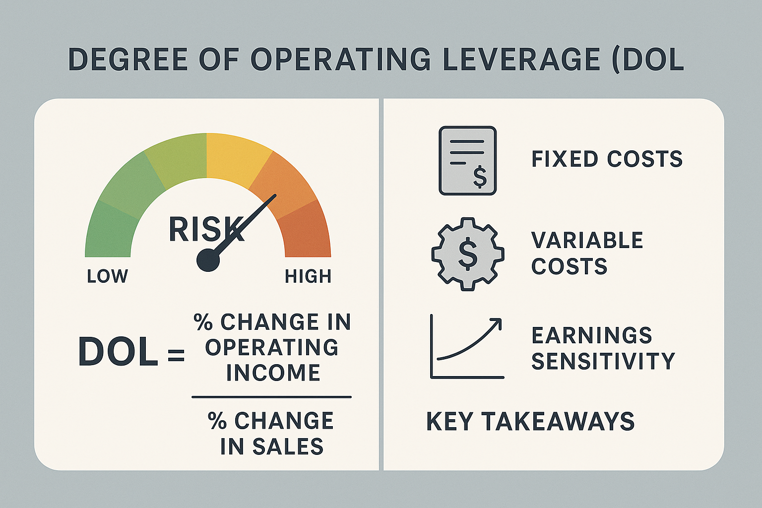
The Degree of Operating Leverage is a financial ratio that measures the percentage change in operating income (EBIT) resulting from a percentage change in sales revenue. It quantifies operational risk by revealing how a company’s cost structure affects profitability.

Operating leverage exists because businesses incur both fixed costs and variable costs. Fixed costs, such as rent, insurance, executive salaries, and depreciation, remain constant regardless of production volume. Variable costs, including raw materials, direct labor, and sales commissions, fluctuate with output levels.

This cost structure creates leverage. Once a company covers its fixed costs, additional sales contribute disproportionately to profit because only variable costs increase. Conversely, when sales decline, fixed costs remain, causing profits to fall faster than revenue.

The Mathematics of Operating Leverage

A company with a DOL of 2.5 will experience a 2.5% change in operating income for every 1% change in sales. This relationship works in both directions:

• Sales increase 10% → Operating income increases 25%
• Sales decrease 10% → Operating income decreases 25%

The amplification effect stems directly from the proportion of fixed costs in the business model. Higher fixed costs create greater leverage, magnifying both upside potential and downside risk.

Consider two companies with identical $1 million in sales:

Company A (Low Operating Leverage):

• Fixed Costs: $200,000
• Variable Costs: $600,000
• Operating Income: $200,000

Company B (High Operating Leverage):

• Fixed Costs: $600,000
• Variable Costs: $200,000
• Operating Income: $200,000

If sales increase 20% to $1.2 million, Company A’s operating income rises to $280,000 (40% increase), while Company B’s jumps to $440,000 (120% increase). The difference? Company B’s cost structure creates significantly higher operating leverage.

This mathematical relationship directly impacts accounting profit and ultimately determines how efficiently a business converts revenue growth into earnings expansion.

How to Calculate Degree of Operating Leverage

Three distinct formulas calculate DOL, each using different available data. All three methods produce the same result when applied correctly, allowing analysts to work with whatever information is accessible.

Method 1: Percentage Change Formula

The most intuitive approach measures the direct relationship between changes in operating income and changes in sales:

DOL = % Change in Operating Income ÷ % Change in Sales

This formula requires two periods of data to calculate the percentage changes.

Example Calculation:

A manufacturing company reports the following:

• Year 1 Sales: $5,000,000 | Operating Income: $800,000
• Year 2 Sales: $5,500,000 | Operating Income: $1,040,000

Step 1: Calculate percentage change in sales

• ($5,500,000 – $5,000,000) ÷ $5,000,000 = 10%

Step 2: Calculate the percentage change in operating income

• ($1,040,000 – $800,000) ÷ $800,000 = 30%

Step 3: Calculate DOL

• 30% ÷ 10% = 3.0

This DOL of 3.0 means operating income changes three times faster than sales revenue, a clear indicator of substantial fixed costs in the business model.

Method 2: Contribution Margin Formula

When single-period data is available, the contribution margin approach provides an efficient calculation:

DOL = Contribution Margin ÷ Operating Income

Where: Contribution Margin = Sales – Variable Costs

Example Calculation:

Using the same company’s Year 2 data:

• Sales: $5,500,000
• Variable Costs: $3,300,000
• Fixed Costs: $1,160,000
• Operating Income: $1,040,000

Step 1: Calculate contribution margin

• $5,500,000 – $3,300,000 = $2,200,000

Step 2: Calculate DOL

• $2,200,000 ÷ $1,040,000 = 2.12

Note: This method calculates DOL at a specific sales level, while the percentage change method measures DOL over a range. The values differ because DOL changes as sales volume changes; it’s not a static metric.

Method 3: Cost Structure Formula

The most comprehensive formula directly incorporates all cost components:

DOL = (Sales – Variable Costs) ÷ (Sales – Variable Costs – Fixed Costs)

This can be simplified to:

DOL = Contribution Margin ÷ Operating Income

This formula is mathematically identical to Method 2 but shows the explicit relationship between fixed costs, variable costs, and leverage.

Example Calculation:

• Sales: $5,500,000
• Variable Costs: $3,300,000
• Fixed Costs: $1,160,000

DOL = ($5,500,000 – $3,300,000) ÷ ($5,500,000 – $3,300,000 – $1,160,000)
DOL = $2,200,000 ÷ $1,040,000 = 2.12

Understanding these calculation methods enables investors to analyze companies using financial statements, where balance sheet basics and cash flow statement data provide the necessary inputs.

Understanding Fixed Costs vs. Variable Costs

The distinction between fixed and variable costs forms the foundation of operating leverage analysis. These cost categories behave fundamentally differently as production volume changes, creating the leverage effect.

Fixed Costs: The Leverage Creator

Fixed costs remain constant regardless of production volume or sales level within a relevant range. These expenses must be paid whether a company produces one unit or one million units.

Common fixed costs include:

• Rent and lease payments for facilities and equipment
• Property insurance and general liability coverage
• Executive salaries and administrative staff compensation
• Depreciation on buildings, machinery, and equipment
• Software licenses and technology infrastructure
• Marketing contracts and annual advertising commitments

Fixed costs create leverage because they establish a baseline expense level. Once sales revenue exceeds this baseline, each additional dollar of revenue contributes more heavily to profit since fixed costs don’t increase.

A software company with $2 million in annual fixed costs (servers, salaries, office space) faces the same expense whether it has 100 customers or 10,000 customers. This cost structure creates enormous profit potential as the customer base grows.

Variable Costs: The Profit Dampener

Variable costs change proportionally with production volume. As output increases, these costs rise; as production decreases, they fall.

Common variable costs include:

• Raw materials and parts
• Direct labor tied to production (hourly wages, piece-rate compensation)
• Sales commissions based on revenue
• Shipping and freight costs
• Packaging materials
• Utilities directly tied to production (electricity for machinery)
• Credit card processing fees (percentage-based)

Variable costs dampen the leverage effect because they consume a portion of each additional sales dollar. A manufacturing company that spends $60 on materials and labor for each $100 product sold retains only $40 contribution margin before fixed costs.

The Leverage Equation

Operating leverage emerges from the relationship between these cost types:

High Fixed Costs + Low Variable Costs = High Operating Leverage
Low Fixed Costs + High Variable Costs = Low Operating Leverage

This relationship directly affects EBITDA and EBITDA margin, as companies with different cost structures show vastly different profitability patterns even at identical revenue levels.

A consulting firm with primarily variable costs (consultant salaries tied to billable hours) has low operating leverage. An airline with massive fixed costs (aircraft leases, airport fees, pilot salaries) has extremely high operating leverage, explaining why airlines swing from huge profits to devastating losses with relatively modest changes in passenger volume.

What Does DOL Tell You About a Business?

The Degree of Operating Leverage reveals three critical insights about a company’s operational characteristics, risk profile, and profit potential.

1. Operational Risk and Profit Volatility

DOL quantifies operational risk by measuring earnings sensitivity to revenue fluctuations. Higher DOL values indicate greater profit volatility and operational risk.

A company with a DOL of 4.0 faces substantial operational risk. A 5% sales decline causes a 20% operating income drop. During economic downturns or competitive pressures, this volatility can be devastating.

Conversely, a company with a DOL of 1.2 shows stable earnings. The same 5% sales decline produces only a 6% profit reduction, manageable and predictable.

This risk assessment informs investment decisions and portfolio construction. Conservative investors seeking stability favor low-DOL companies. Growth investors willing to accept volatility target high-DOL companies with strong revenue growth prospects.

The relationship between operating leverage and financial risk parallels concepts in risk management, where understanding volatility enables better decision-making.

2. Cost Structure and Business Model

DOL reveals cost structure without detailed expense breakdowns. A high DOL immediately signals a business model built on fixed costs and economies of scale.

Consider these DOL interpretations:

• DOL = 1.5 to 2.5: Moderate fixed costs, balanced business model
• DOL = 3.0 to 5.0: Significant fixed costs, capital-intensive operations
• DOL > 5.0: Extremely high fixed costs, substantial operational leverage

A software-as-a-service (SaaS) company with a DOL of 4.5 clearly operates on high fixed costs (development, infrastructure) and low variable costs (customer support). This structure creates powerful profit expansion as the customer base grows.

A retail company with a DOL of 1.8 shows higher variable costs (inventory, sales staff) relative to fixed costs, a fundamentally different business model with different profit characteristics.

3. Profit Potential and Scalability

DOL indicates scalability and profit expansion potential. High operating leverage companies can achieve explosive profit growth when sales increase because fixed costs remain constant.

A manufacturing company with a DOL of 5.0 that increases sales by 20% will see operating income surge by 100%. This mathematical relationship explains why high-leverage companies command premium valuations during growth phases.

However, this same leverage works in reverse. The same company experiencing a 20% sales decline faces a catastrophic 100% operating income collapse.

This dual nature of operating leverage, amplifying both gains and losses, makes DOL essential for understanding earnings per share volatility and predicting future profitability under different revenue scenarios.

Insight: Operating leverage transforms revenue changes into magnified profit changes. Understanding this amplification effect enables investors to predict earnings volatility, assess operational risk, and identify companies positioned for explosive profit growth during expansion phases.

DOL Across Different Industries

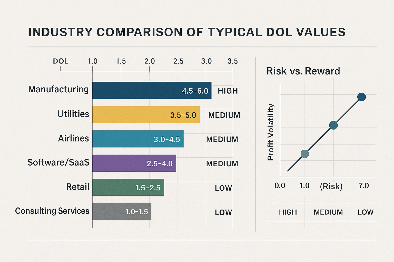
Operating leverage varies dramatically across industries based on inherent business model characteristics. Capital-intensive industries naturally exhibit higher DOL than service-based businesses.

High Operating Leverage Industries

Manufacturing (DOL typically 4.0-6.0)

Manufacturing companies invest heavily in factories, equipment, and production infrastructure. These fixed assets create substantial depreciation and maintenance costs that remain constant regardless of production volume.

An automotive manufacturer with $500 million in annual fixed costs (factory leases, equipment depreciation, engineering salaries) and $300 per vehicle in variable costs shows extreme operating leverage. Selling 100,000 additional vehicles dramatically impacts profitability because fixed costs don’t increase.

Airlines (DOL typically 3.5-5.5)

Airlines face enormous fixed costs: aircraft leases, airport gate fees, pilot and crew salaries, maintenance facilities, and reservation systems. Variable costs (fuel, in-flight meals, and landing fees) represent a smaller proportion of total expenses.

This cost structure explains airline industry volatility. A 10% passenger volume increase can double profits, while a 10% decrease can eliminate profitability, the mathematics of high operating leverage in action.

Utilities (DOL typically 3.0-5.0)

Electric, gas, and water utilities operate massive infrastructure networks requiring constant maintenance. Power plants, transmission lines, and distribution systems create substantial fixed costs regardless of consumption levels.

Telecommunications (DOL typically 2.5-4.0)

Network infrastructure, cell towers, fiber optic cables, and data centers represent huge fixed investments. Once built, serving additional customers requires minimal incremental cost, creating significant operating leverage.

Moderate Operating Leverage Industries

Software and SaaS (DOL typically 2.0-4.0)

Software companies show interesting leverage characteristics. Development costs are fixed (engineering salaries, infrastructure), but customer acquisition costs can be substantial. The balance between these factors determines overall leverage.

Established software companies with strong brand recognition show higher leverage than startups that spend heavily on customer acquisition.

Retail (DOL typically 1.5-2.5)

Retailers balance fixed costs (store leases, corporate overhead) with substantial variable costs (inventory, sales staff). This creates moderate operating leverage—enough to benefit from sales growth but not enough to create extreme volatility.

Low Operating Leverage Industries

Consulting and Professional Services (DOL typically 1.0-2.0)

Service businesses built on billable hours show low operating leverage. Consultant salaries, the primary expense, scale with revenue. Fixed costs (office space, administrative staff) represent a smaller proportion of total expenses.

This cost structure creates stability but limits profit expansion potential during growth phases.

Restaurants (DOL typically 1.2-2.0)

Food costs, hourly labor, and supplies represent substantial variable expenses. While rent and management salaries are fixed, the high proportion of variable costs reduces overall leverage.

Industry Comparison Implications

Understanding industry-typical DOL values enables meaningful analysis:

1. Compare companies within industries, not across industries
2. Expect higher volatility from high-leverage sectors during economic cycles
3. Recognize profit potential in high-DOL companies during expansion
4. Value stability in low-DOL companies during uncertainty

This industry context complements the analysis of efficiency ratios and capitalization ratios, providing a comprehensive view of operational and financial characteristics.

Operating Leverage and Break-Even Analysis

Operating leverage directly determines break-even dynamics and the speed at which companies transition from losses to profits as sales volume increases.

The Break-Even Point

The break-even point occurs when total revenue equals total costs (fixed plus variable), resulting in zero operating income.

Break-Even Sales = Fixed Costs ÷ Contribution Margin Ratio

Where: Contribution Margin Ratio = (Sales – Variable Costs) ÷ Sales

Operating leverage affects how quickly companies move beyond break-even. High-leverage companies require higher sales volumes to break even due to substantial fixed costs, but they achieve rapid profit acceleration once that threshold is crossed.

Example: Two Business Models

Company A (High Operating Leverage):

• Fixed Costs: $800,000
• Variable Costs: 30% of sales
• Contribution Margin Ratio: 70%
• Break-Even Sales: $800,000 ÷ 0.70 = $1,142,857

Company B (Low Operating Leverage):

• Fixed Costs: $300,000
• Variable Costs: 70% of sales
• Contribution Margin Ratio: 30%
• Break-Even Sales: $300,000 ÷ 0.30 = $1,000,000

Company B reaches break-even at a lower sales volume, but Company A generates profit faster beyond break-even:

At $1,500,000 in sales:

• Company A: Operating Income = ($1,500,000 × 0.70) – $800,000 = $250,000
• Company B: Operating Income = ($1,500,000 × 0.30) – $300,000 = $150,000

Company A produces 67% more profit at the same revenue level due to higher operating leverage.

The Margin of Safety

Margin of safety measures how far sales can decline before reaching break-even:

Margin of Safety = (Current Sales – Break-Even Sales) ÷ Current Sales

High operating leverage companies typically show lower margins of safety, indicating greater vulnerability to sales declines. This relationship quantifies operational risk and informs budget planning and stress testing.

A company with $2 million in sales and $1.6 million break-even point has only a 20% margin of safety. A 25% sales decline would push the company into losses, a precarious position requiring careful monitoring.

Strategic Implications

Understanding the operating leverage-break-even relationship guides strategic decisions:

1. Capital investment decisions: High fixed-cost investments increase leverage and break-even points
2. Pricing strategies: High-leverage companies benefit more from price increases than volume increases
3. Cost structure optimization: Balancing fixed and variable costs affects both risk and profit potential
4. Capacity planning: Operating leverage determines optimal capacity utilization

This analysis connects to broader financial planning concepts, including the 50/30/20 rule budgeting framework for personal finances and the 4% rule for retirement planning—all examples of mathematical relationships that drive financial decisions.

Limitations and Considerations

While DOL provides valuable insights, several limitations require careful consideration when applying this metric to investment analysis and business evaluation.

1. DOL Changes with Sales Volume

Operating leverage is not constant. It changes as sales volume moves closer to or further from the break-even point.

At sales levels near break-even, DOL is extremely high because operating income is small. A small percentage change in sales creates enormous percentage changes in the small operating income base.

As sales increase well beyond break-even, DOL decreases because operating income becomes larger relative to contribution margin. The same absolute profit change represents a smaller percentage change.

Example:

A company with $1 million contribution margin shows different DOL at different profit levels:

• At $100,000 operating income: DOL = $1,000,000 ÷ $100,000 = 10.0
• At $500,000 operating income: DOL = $1,000,000 ÷ $500,000 = 2.0
• At $900,000 operating income: DOL = $1,000,000 ÷ $900,000 = 1.11

This changing relationship means DOL calculations reflect specific points in time and sales volumes, not universal company characteristics.

2. Fixed Costs Aren’t Truly Fixed

“Fixed” costs eventually change with significant volume shifts or strategic decisions.

A manufacturing company operating at 60% capacity can increase production without adding factory space. But expanding from 90% to 120% capacity requires new facilities, equipment, and supervisors—converting “fixed” costs into step-function costs.

Similarly, companies can reduce fixed costs during sustained downturns through facility closures, workforce reductions, and contract renegotiations. The fixed-variable distinction holds only within relevant ranges.

3. Accounting Classifications Vary

Different accounting methods classify costs differently, affecting DOL calculations.

Some companies classify certain labor costs as fixed (salaried employees), while others treat similar costs as variable (hourly workers). Depreciation methods, lease accounting, and overhead allocation all impact the fixed-variable split.

This variation makes cross-company comparisons challenging unless analysts adjust for accounting differences. Understanding cash vs accrual accounting helps identify these classification issues.

4. Operating Leverage vs. Financial Leverage

Operating leverage differs from financial leverage, though both amplify returns.

Operating leverage stems from fixed operating costs and affects EBIT’s sensitivity to sales changes. Financial leverage results from debt financing and affects net income sensitivity to EBIT changes.

Combined leverage (operating leverage × financial leverage) determines how sales changes affect earnings per share. A company with high operating leverage and high financial leverage shows extreme earnings volatility—a critical consideration for risk assessment.

The debt-to-equity ratio and equity ratio measure financial leverage, complementing operating leverage analysis for comprehensive risk evaluation.

5. External Factors Override Internal Leverage

Market conditions and competitive dynamics can overwhelm operating leverage effects.

A company with favorable operating leverage still suffers during industry downturns, technological disruption, or competitive pressure. DOL measures internal operational characteristics, not external market forces.

Investors must combine operating leverage analysis with industry analysis, competitive positioning, and macroeconomic assessment for a complete evaluation.

6. Service Quality and Customer Satisfaction

Cost structure optimization can harm long-term competitiveness.

Companies might reduce variable costs (customer service, product quality, employee training) to increase operating leverage and short-term profit margins. This strategy risks customer satisfaction, brand reputation, and sustainable competitive advantage.

The mathematics of operating leverage reveal profit sensitivity, but they don’t capture strategic positioning or long-term value creation.

Takeaway: Operating leverage provides powerful insights into profit dynamics and operational risk, but it represents one analytical tool among many. Effective investment analysis combines DOL with industry context, competitive analysis, financial leverage assessment, and qualitative business evaluation.

Practical Applications for Investors

Understanding operating leverage transforms from an academic concept to a practical investment tool when applied to real-world analysis and decision-making.

1. Earnings Volatility Prediction

DOL enables earnings forecasting under different revenue scenarios.

An investor analyzing a company with a DOL of 3.5 can model earnings outcomes:

• Bull case (20% revenue growth): Operating income increases 70%
• Base case (10% revenue growth): Operating income increases 35%
• Bear case (5% revenue decline): Operating income decreases 17.5%

This scenario analysis quantifies risk-reward trade-offs and informs position sizing. High-conviction investors might overweight high-DOL companies in growth portfolios, while conservative investors might limit exposure due to downside volatility.

2. Sector Rotation Strategies

Operating leverage guides sector allocation across economic cycles.

During early economic recovery, high-leverage sectors (manufacturing, airlines, industrials) offer disproportionate profit growth as revenue recovers. Investors rotating into these sectors early in expansion cycles capture amplified earnings growth.

During late-cycle periods or economic uncertainty, rotating toward low-leverage sectors (consumer staples, utilities, healthcare) reduces portfolio volatility and preserves capital.

This tactical approach complements diversification investing strategies and enhances risk-adjusted returns.

3. Valuation Context

DOL affects appropriate valuation multiples.

High operating leverage companies trading at 15x earnings during mid-cycle conditions might deserve premium valuations if revenue growth accelerates. The same multiple might be expensive for low-leverage companies with limited profit expansion potential.

Conversely, high-DOL companies warrant valuation discounts during uncertain periods due to downside earnings risk.

Understanding this relationship improves enterprise value analysis and prevents valuation errors based on superficial multiple comparisons.

4. Competitive Advantage Assessment

Cost structure reveals competitive positioning and strategic flexibility.

Companies with low operating leverage maintain flexibility to adjust costs during downturns, providing competitive advantages during industry stress. High-leverage competitors face fixed cost burdens that force difficult decisions during revenue declines.

However, high-leverage companies with sustainable competitive advantages (brand strength, network effects, regulatory protection) can leverage fixed-cost structures into dominant profit margins during normal conditions.

This analysis complements traditional competitive moat assessment and identifies companies positioned for long-term outperformance.

5. Management Quality Evaluation

Operating leverage trends reveal management decisions about cost structure and strategic positioning.

Increasing DOL over time indicates management investing in fixed assets, automation, and infrastructure—signaling confidence in future growth and willingness to accept operational risk for profit potential.

Decreasing DOL suggests management prioritizing flexibility and risk reduction over profit maximization—appropriate during uncertainty but potentially indicating limited growth ambitions.

Tracking DOL changes alongside capital allocation strategies provides insight into management quality and strategic direction.

6. Risk-Adjusted Portfolio Construction

DOL informs position sizing and portfolio risk management.

A portfolio containing multiple high-leverage companies in cyclical industries concentrates operational risk. During economic downturns, these positions simultaneously experience magnified earnings declines.

Balancing high-DOL growth positions with low-DOL stable positions creates portfolio resilience across economic conditions. This approach mirrors the principles in the 3x rent rule and 20/4/10 rule car buying—mathematical frameworks that manage risk through balanced allocation.

Real-World Example: Operating Leverage in Action

Consider two hypothetical companies in the same industry to illustrate operating leverage effects across different scenarios.

Company Profiles

TechManufacture Inc. (High Operating Leverage)

• Annual Sales: $10,000,000
• Fixed Costs: $6,000,000 (factory, equipment, salaried staff)
• Variable Costs: $2,000,000 (materials, hourly labor)
• Operating Income: $2,000,000
• DOL = $8,000,000 ÷ $2,000,000 = 4.0

FlexiProd Corp. (Low Operating Leverage)

• Annual Sales: $10,000,000
• Fixed Costs: $2,000,000 (minimal infrastructure)
• Variable Costs: $6,000,000 (outsourced production, contract labor)
• Operating Income: $2,000,000
• DOL = $4,000,000 ÷ $2,000,000 = 2.0

Both companies generate identical revenue and operating income, but their cost structures create vastly different profit dynamics.

Scenario 1: 20% Revenue Growth

TechManufacture Inc.:

• New Sales: $12,000,000
• Fixed Costs: $6,000,000 (unchanged)
• Variable Costs: $2,400,000 (20% increase)
• Operating Income: $3,600,000
• Operating Income Growth: 80% (4.0 DOL × 20% sales growth)

FlexiProd Corp.:

• New Sales: $12,000,000
• Fixed Costs: $2,000,000 (unchanged)
• Variable Costs: $7,200,000 (20% increase)
• Operating Income: $2,800,000
• Operating Income Growth: 40% (2.0 DOL × 20% sales growth)

TechManufacture’s operating leverage produces double the profit growth of FlexiProd from identical revenue increases.

Scenario 2: 15% Revenue Decline

TechManufacture Inc.:

• New Sales: $8,500,000
• Fixed Costs: $6,000,000 (unchanged)
• Variable Costs: $1,700,000 (15% decrease)
• Operating Income: $800,000
• Operating Income Decline: 60% (4.0 DOL × 15% sales decline)

FlexiProd Corp.:

• New Sales: $8,500,000
• Fixed Costs: $2,000,000 (unchanged)
• Variable Costs: $5,100,000 (15% decrease)
• Operating Income: $1,400,000
• Operating Income Decline: 30% (2.0 DOL × 15% sales decline)

TechManufacture’s high leverage creates severe profit compression during downturns, while FlexiProd maintains relative stability.

Investment Implications

Growth Environment: TechManufacture offers superior profit expansion potential, justifying higher valuation multiples and larger portfolio positions for growth-oriented investors.

Uncertain Environment: FlexiProd provides defensive characteristics and earnings stability, appropriate for risk-averse investors or late-cycle positioning.

Valuation Adjustment: If both companies trade at 15x earnings ($30 million market cap), TechManufacture appears undervalued in growth scenarios but overvalued in decline scenarios. Context determines appropriate valuation.

This example demonstrates why understanding operating leverage is essential for data-driven investment decisions, complementing analysis of absolute return and annualized return metrics.

Conclusion

The Degree of Operating Leverage reveals the mathematical relationship between sales changes and profit changes, quantifying how a company's cost structure amplifies earnings volatility. This metric transforms abstract concepts of fixed and variable costs into concrete measurements of operational risk and profit potential.

High operating leverage creates opportunity and danger. Companies with substantial fixed costs generate explosive profit growth during expansion but face severe profit compression during downturns. Low operating leverage provides stability and flexibility but limits profit expansion potential even during strong growth periods.

Understanding DOL enables data-driven investment decisions grounded in operational reality rather than superficial financial metrics. Investors who incorporate operating leverage analysis into their evaluation process gain insight into:

• Earnings volatility and the range of potential outcomes under different scenarios
• Operational risk stemming from cost structure and business model choices
• Profit potential during growth phases based on leverage amplification
• Competitive positioning revealed through cost structure analysis
• Management quality is demonstrated by strategic cost structure decisions

The math behind operating leverage demonstrates a fundamental truth: business models matter. Two companies with identical revenue and current profitability can show vastly different future profit trajectories based solely on their fixed-to-variable cost ratios.

Next Steps

Apply operating leverage analysis to your investment process:

1. Calculate DOL for companies in your portfolio or watchlist using financial statement data
2. Compare leverage within industries to identify outliers and understand competitive dynamics
3. Model scenarios showing profit outcomes under different revenue growth assumptions
4. Assess risk tolerance and adjust portfolio positions based on operating leverage exposure
5. Monitor trends in company DOL over time to identify strategic shifts and changing risk profiles

Operating leverage represents one component of comprehensive financial analysis. Combine DOL insights with balance sheet basics, cash flow analysis, valuation metrics, and competitive assessment for complete investment evaluation.

The companies that thrive over decades understand their operating leverage and manage it strategically. As an investor, understanding this same mathematics provides an analytical edge—the ability to predict earnings trajectories, assess operational risk, and make evidence-based allocation decisions that compound wealth over time.

References

[1] Corporate Finance Institute - Operating Leverage (corporatefinanceinstitute.com)

[2] CFA Institute - Cost Behavior and Operating Leverage (cfainstitute.org)

[3] Financial Accounting Standards Board - Cost Classification Guidelines (fasb.org)

[4] Harvard Business Review - Understanding Business Model Economics (hbr.org)

[5] Journal of Financial Economics - Operating Leverage and Stock Returns (sciencedirect.com)

Author Bio

Max Fonji is a data-driven financial educator and the voice behind The Rich Guy Math. With expertise in financial analysis, valuation principles, and evidence-based investing, Max translates complex financial concepts into clear, actionable insights. His analytical approach combines rigorous mathematics with practical application, helping investors understand the cause-and-effect relationships that drive wealth building and long-term financial success.

Educational Disclaimer

This article provides educational information about the Degree of Operating Leverage and financial analysis concepts. It does not constitute investment advice, financial planning guidance, or recommendations to buy or sell securities. Operating leverage analysis represents one analytical tool among many and should be combined with comprehensive research, risk assessment, and professional consultation before making investment decisions.

Financial metrics and ratios reflect historical data and current conditions; they do not guarantee future performance. All investments carry risk, including potential loss of principal. Investors should conduct thorough due diligence, consider their individual financial circumstances and risk tolerance, and consult qualified financial advisors before making investment decisions.

The examples and calculations presented are for educational illustration only and do not represent actual companies or investment recommendations. Individual results will vary based on specific company circumstances, market conditions, and numerous other factors.