Every business decision carries a multiplier effect that most investors overlook. When a company increases sales by 10%, earnings might jump 30%, or collapse by the same amount. This amplification isn’t magic; it’s Combined Leverage, the mathematical relationship between operating structure and financing choices that determines how sensitive profits are to revenue changes.
Understanding Combined Leverage reveals the math behind money at the corporate level. It explains why some companies deliver explosive returns during growth periods while others face catastrophic losses during downturns. For investors seeking data-driven insights into risk management and return potential, this concept provides a quantifiable framework for evaluating business risk.
This guide breaks down Combined Leverage into its core components, demonstrates the formulas with real examples, and shows how this leverage impacts both corporate strategy and investment decisions.
Key Takeaways
- Combined Leverage measures total profit sensitivity to sales changes by multiplying operating leverage and financial leverage together.
- The formula (DCL = DOL × DFL) quantifies how a percentage change in sales translates to a percentage change in earnings per share.
- Higher combined leverage amplifies both gains and losses, creating greater return potential with proportionally greater risk.
- Operating leverage stems from fixed costs in the business model, while financial leverage comes from debt in the capital structure.
- Investors can use DCL to compare risk profiles across companies and industries, making more informed capital allocation decisions.
What Is Combined Leverage? The Foundation Explained
Combined Leverage represents the total amplification effect on earnings per share (EPS) resulting from changes in sales revenue. It combines two distinct types of leverage, operating leverage and financial leverage, into a single multiplier that reveals a company’s complete risk-return profile.
Operating leverage measures how fixed costs in a business model magnify changes in sales into larger changes in operating income (EBIT). A company with high fixed costs and low variable costs has high operating leverage.
Financial leverage measures how debt in the capital structure magnifies changes in operating income into larger changes in earnings available to shareholders. A company with significant debt has high financial leverage.
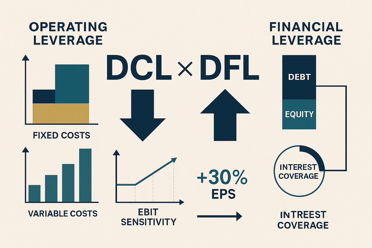
When these two forces combine, they create a compounding effect. A 10% increase in sales might lead to a 15% increase in EBIT (due to operating leverage), which then translates to a 25% increase in EPS (due to financial leverage). The Combined Leverage captures this entire chain reaction in one metric.
The Mathematical Formula
The Degree of Combined Leverage (DCL) uses this formula:
DCL = DOL × DFL
Where:
- DCL = Degree of Combined Leverage
- DOL = Degree of Operating Leverage
- DFL = Degree of Financial Leverage
Alternatively, DCL can be calculated directly as:
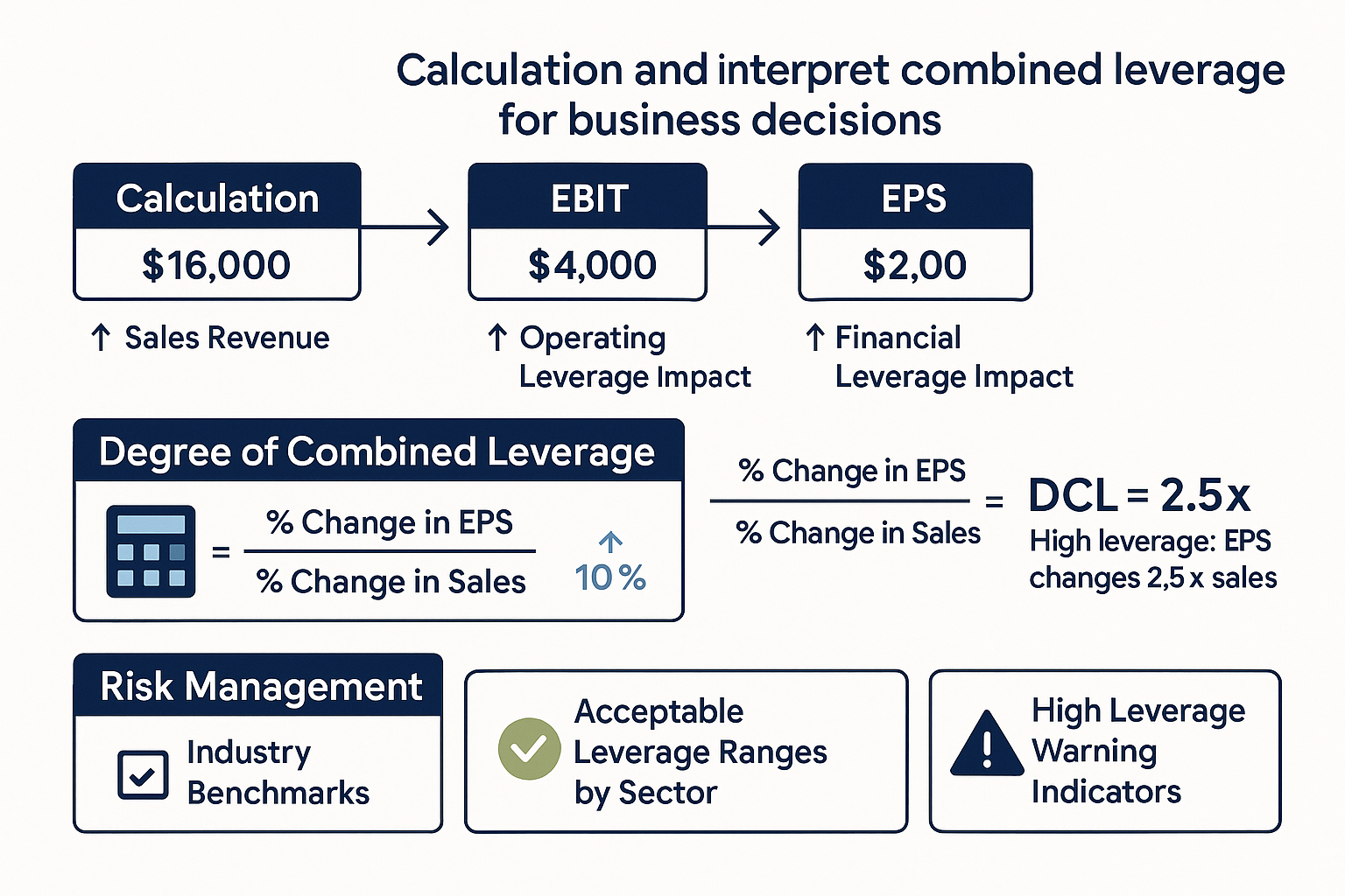
DCL = % Change in EPS / % Change in Sales
This ratio tells investors exactly how much earnings per share will change for each 1% change in sales revenue. A DCL of 3.0 means that a 10% sales increase produces a 30% EPS increase, and a 10% sales decrease produces a 30% EPS decrease.
Why This Matters for Investors
Combined Leverage provides a quantifiable measure of business risk. Companies with high DCL offer greater return potential during economic expansions but face steeper losses during contractions. This knowledge enables evidence-based investing decisions aligned with risk tolerance and market conditions.
Understanding leverage helps investors avoid companies with unsustainable risk profiles while identifying opportunities where calculated risk offers asymmetric returns. The math reveals what qualitative analysis might miss.
Operating Leverage: The First Component of Combined Leverage
Operating leverage exists because of the relationship between fixed costs and variable costs in a company’s cost structure. Fixed costs, like rent, salaries, equipment depreciation, and insurance, remain constant regardless of production volume. Variable costs, like raw materials, direct labor, and sales commissions, change proportionally with output.
When a company has high fixed costs relative to variable costs, small changes in sales volume create larger changes in operating profit. This happens because once fixed costs are covered, additional revenue flows more directly to profit.
The Operating Leverage Formula
DOL = % Change in EBIT / % Change in Sales
Or, calculated at a specific sales level:
DOL = [Q(P – V)] / [Q(P – V) – F]
Where:
- Q = Quantity of units sold
- P = Price per unit
- V = Variable cost per unit
- F = Fixed costs
A simpler calculation method:
DOL = Contribution Margin / Operating Income
Where Contribution Margin = Sales – Variable Costs
Real-World Example: Software vs Manufacturing
Consider two companies, each with $1 million in sales:
Software Company:
- Fixed costs: $600,000 (salaries, servers, office)
- Variable costs: $100,000 (customer support, hosting)
- EBIT: $300,000
- DOL = ($1M – $100K) / $300K = 3.0
Manufacturing Company:
- Fixed costs: $200,000 (facility, equipment)
- Variable costs: $600,000 (materials, direct labor)
- EBIT: $200,000
- DOL = ($1M – $600K) / $200K = 2.0
If both companies increase sales by 20% to $1.2 million:
Software Company:
- New EBIT: $480,000 (60% increase)
- Variable costs only increased by $20,000
Manufacturing Company:
- New EBIT: $280,000 (40% increase)
- Variable costs increased by $120,000
The software company’s higher operating leverage amplified the sales increase into a larger profit increase. This same leverage works in reverse during downturns, making high operating leverage a double-edged sword.
Industry Patterns in Operating Leverage
Different industries naturally exhibit different levels of operating leverage:
High Operating Leverage Industries:
- Software and SaaS (minimal marginal costs)
- Airlines (high fixed costs for planes and staff)
- Hotels (fixed property and maintenance costs)
- Telecommunications (infrastructure-heavy)
Low Operating Leverage Industries:
- Retail (inventory costs scale with sales)
- Consulting (variable labor costs)
- Wholesale distribution (variable product costs)
- Food services (ingredient costs vary with volume)
Investors evaluating accounting profit should recognize that companies with high operating leverage show greater profit volatility, which affects valuation multiples and risk assessment.
Financial Leverage: The Second Component of Combined Leverage
Financial leverage arises from the use of debt in a company’s capital structure. When a company borrows money, it commits to fixed interest payments regardless of operating performance. This creates a similar amplification effect to operating leverage, but at a different level of the income statement.
Interest payments are fixed obligations that must be paid before any earnings flow to shareholders. When operating income increases, the fixed interest expense stays constant, allowing a larger percentage increase in earnings available to equity holders. Conversely, declining operating income combined with fixed interest creates magnified losses for shareholders.
The Financial Leverage Formula
DFL = % Change in EPS / % Change in EBIT
Or, calculated at a specific EBIT level:
DFL = EBIT / (EBIT – Interest Expense)
This formula shows how sensitive earnings per share are to changes in operating income. A DFL of 2.0 means that a 10% change in EBIT produces a 20% change in EPS.
Numerical Example: Impact of Debt
Compare two identical companies with different capital structures:
Company A (No Debt):
- EBIT: $500,000
- Interest expense: $0
- Earnings before tax: $500,000
- Tax (25%): $125,000
- Net income: $375,000
- Shares outstanding: 100,000
- EPS: $3.75
- DFL = $500,000 / ($500,000 – $0) = 1.0
Company B (With Debt):
- EBIT: $500,000
- Interest expense: $150,000
- Earnings before tax: $350,000
- Tax (25%): $87,500
- Net income: $262,500
- Shares outstanding: 70,000 (fewer shares due to debt financing)
- EPS: $3.75
- DFL = $500,000 / ($500,000 – $150,000) = 1.43
Both companies currently show the same EPS, but watch what happens when EBIT increases by 20% to $600,000:
Company A:
- New net income: $450,000
- New EPS: $4.50 (20% increase)
Company B:
- New earnings before tax: $450,000
- New net income: $337,500
- New EPS: $4.82 (28.5% increase)
Company B’s financial leverage amplified the 20% EBIT increase into a 28.5% EPS increase. This demonstrates why debt can enhance returns to equity holders during growth periods.
The Risk Side of Financial Leverage
The same leverage works destructively during downturns. If EBIT decreases by 20% to $400,000:
Company A:
- New EPS: $3.00 (20% decrease)
Company B:
- New earnings before tax: $250,000
- New net income: $187,500
- New EPS: $2.68 (28.5% decrease)
Financial leverage magnifies both gains and losses symmetrically. This is why highly leveraged companies experience greater stock price volatility and carry higher risk profiles.
Understanding the debt-to-equity ratio and interest coverage metrics helps investors assess whether a company’s financial leverage is sustainable or dangerous.
Calculating Combined Leverage: Putting It All Together
Combined Leverage multiplies the effects of operating leverage and financial leverage to show the total amplification from sales to earnings per share. This calculation provides the complete picture of how business structure and financing decisions interact to create risk and return potential.
The Complete Formula
DCL = DOL × DFL
Using the formulas from previous sections:
DCL = [Q(P – V) / Q(P – V) – F] × [EBIT / (EBIT – Interest)]
Or more simply:
DCL = % Change in EPS / % Change in Sales
Comprehensive Example: Three Leverage Scenarios
Consider three companies in the same industry, each with $2 million in annual sales but different leverage profiles:
Company Low-Lev:
- Fixed costs: $400,000
- Variable costs: $1,200,000
- EBIT: $400,000
- Interest expense: $0
- Net income (after 25% tax): $300,000
- Shares: 100,000
- EPS: $3.00
- DOL = 2.0
- DFL = 1.0
- DCL = 2.0
Company Mid-Lev:
- Fixed costs: $800,000
- Variable costs: $800,000
- EBIT: $400,000
- Interest expense: $100,000
- Net income (after 25% tax): $225,000
- Shares: 75,000
- EPS: $3.00
- DOL = 3.0
- DFL = 1.33
- DCL = 4.0
Company High-Lev:
- Fixed costs: $1,000,000
- Variable costs: $600,000
- EBIT: $400,000
- Interest expense: $200,000
- Net income (after 25% tax): $150,000
- Shares: 50,000
- EPS: $3.00
- DOL = 3.5
- DFL = 2.0
- DCL = 7.0
All three companies currently show the same EPS of $3.00, but their sensitivity to sales changes differs dramatically.
Impact of a 15% Sales Increase
When sales increase 15% to $2.3 million:
Company Low-Lev:
- New EBIT: $520,000 (30% increase)
- New EPS: $3.90 (30% increase)
- Actual DCL = 30% / 15% = 2.0 ✓
Company Mid-Lev:
- New EBIT: $580,000 (45% increase)
- New EPS: $4.80 (60% increase)
- Actual DCL = 60% / 15% = 4.0 ✓
Company High-Lev:
- New EBIT: $610,000 (52.5% increase)
- New EPS: $6.15 (105% increase)
- Actual DCL = 105% / 15% = 7.0 ✓
Company High-Lev delivered a 105% EPS increase from just a 15% sales increase, a spectacular amplification. This explains why high-leverage companies can generate extraordinary returns during favorable conditions.
Impact of a 15% Sales Decrease
The leverage works equally powerfully in reverse. When sales decrease 15% to $1.7 million:
Company Low-Lev:
- New EPS: $2.10 (30% decrease)
Company Mid-Lev:
- New EPS: $1.20 (60% decrease)
Company High-Lev:
- New EPS: -$0.15 (105% decrease, now unprofitable)
Company High-Lev went from $3.00 per share to a loss, while Company Low-Lev remained profitable despite the same sales decline. This illustrates why Combined Leverage is fundamentally a risk metric, not just a return enhancer.
Investors focused on risk management must weigh the potential for amplified returns against the risk of amplified losses when evaluating companies with different leverage profiles.
How Combined Leverage Impacts Investment Risk and Returns
Combined Leverage creates a direct mathematical relationship between business volatility and investment outcomes. Understanding this relationship enables investors to match their portfolio selections with their risk tolerance and market outlook.
The Risk-Return Tradeoff
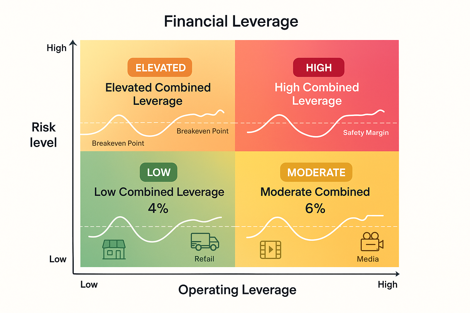
Higher Combined Leverage increases both potential returns and potential losses proportionally. This creates a risk-return spectrum:
| DCL Range | Risk Level | Return Potential | Suitable For |
|---|---|---|---|
| 1.0 – 2.0 | Low | Modest | Conservative investors, stable income seekers |
| 2.0 – 4.0 | Moderate | Good | Balanced portfolios, long-term growth |
| 4.0 – 6.0 | Elevated | High | Growth investors, cyclical opportunities |
| 6.0+ | Very High | Extreme | Aggressive investors, short-term traders |
Companies with DCL above 6.0 should be considered speculative investments. A 10% revenue miss can translate to a 60%+ earnings decline, often triggering severe stock price corrections.
Cyclical Sensitivity
Combined Leverage explains why certain stocks dramatically outperform or underperform during different economic cycles:
During Economic Expansions:
- High-leverage companies capture disproportionate profit growth
- Stock prices often appreciate faster than the broader market
- Valuation multiples expand as growth accelerates
- Investors reward the amplified earnings growth
During Economic Contractions:
- High-leverage companies experience severe profit declines
- Stock prices fall faster than the broader market
- Valuation multiples compress as losses mount
- Investors flee the amplified earnings risk
This cyclical pattern creates opportunities for investors who can correctly time economic cycles, but it also creates substantial risk for those who hold high-leverage companies through downturns.
Sector Variations in Combined Leverage
Different sectors exhibit characteristic Combined Leverage profiles based on their business models and capital intensity:
High Combined Leverage Sectors:
- Airlines: High fixed costs (planes, staff) + high debt (capital-intensive)
- Automotive: Manufacturing fixed costs + inventory financing
- Real Estate Development: Property costs + construction debt
- Semiconductors: Fabrication facilities + R&D costs + equipment financing
Moderate Combined Leverage Sectors:
- Technology: Software has high DOL but often low DFL
- Pharmaceuticals: R&D fixed costs with variable manufacturing costs
- Telecommunications: Infrastructure costs with moderate debt
- Utilities: Regulated returns limit extreme leverage effects
Low Combined Leverage Sectors:
- Professional Services: Variable labor costs, minimal debt
- Retail: Inventory scales with sales, conservative financing
- Consumer Staples: Stable demand reduces operating leverage impact
- Healthcare Services: Relatively stable revenue, moderate fixed costs
Investors building diversified portfolios should consider the Combined Leverage profile of each sector to balance overall portfolio risk. A portfolio concentrated in high-leverage sectors will experience greater volatility than one balanced across the leverage spectrum.
Valuation Implications
Combined Leverage directly affects appropriate valuation multiples. Companies with high DCL should theoretically trade at lower price-to-earnings ratios because of their elevated risk profiles. The market often violates this principle during bull markets, creating overvaluation in high-leverage names.
A rational valuation framework adjusts for leverage risk:
- Low DCL (1-2): Can support P/E ratios of 20-25x in growth scenarios
- Moderate DCL (2-4): Appropriate P/E ratios of 15-20x
- High DCL (4-6): Should trade at P/E ratios of 10-15x
- Very High DCL (6+): Requires P/E ratios below 10x to compensate for risk
When high-leverage companies trade at premium valuations, they carry double risk: operational leverage plus valuation compression risk. This combination explains the spectacular crashes of overleveraged companies during market corrections.
Understanding enterprise value and equity valuation principles helps investors assess whether a company’s stock price appropriately reflects its leverage risk.
Strategic Applications: Using Combined Leverage in Decision-Making
Both corporate managers and investors can apply the Combined Leverage analysis to make better strategic decisions. The framework provides quantifiable insights into risk-return tradeoffs that qualitative analysis alone cannot reveal.
For Corporate Strategy
Capacity Planning:
Companies can model how different fixed cost investments (new facilities, equipment, technology platforms) will affect operating leverage and overall risk profile. A $10 million investment in automation might increase DOL from 2.5 to 4.0, which, combined with existing financial leverage, could push DCL above acceptable risk thresholds.
Capital Structure Decisions:
CFOs can calculate the impact of debt financing on Combined Leverage before making borrowing decisions. If a company already has high operating leverage (DOL of 4.0), adding significant debt that increases DFL from 1.2 to 2.0 would push DCL from 4.8 to 8.0—potentially creating unsustainable risk.
Pricing Strategy:
Understanding leverage helps companies set prices appropriately. High-leverage companies need higher profit margins to create adequate safety buffers, while low-leverage companies can compete more aggressively on price.
Risk Management:
Companies can use DCL to determine appropriate cash reserves and credit facilities. A company with a DCL of 6.0 needs larger emergency funds than one with a DCL of 2.0 because the same revenue decline creates three times the earnings impact.
For Investment Analysis
Stock Selection:
Investors can screen for companies with Combined Leverage profiles matching their risk tolerance. Conservative investors might filter for DCL below 3.0, while aggressive growth investors might seek DCL of 5.0+ in expanding industries.
Portfolio Construction:
Building a balanced portfolio requires mixing leverage profiles. A portfolio of ten stocks with an average DCL of 6.0 will experience roughly twice the volatility of a portfolio with an average DCL of 3.0. Investors can target specific portfolio-level leverage by blending high and low DCL positions.
Timing Decisions:
Combined Leverage analysis helps with market timing. Early in economic expansions, high-leverage stocks often outperform. Late in expansions or during contractions, shifting to low-leverage stocks reduces portfolio risk. This approach aligns with the cycle of market emotions that drives investor behavior.
Risk-Adjusted Returns:
Comparing returns without adjusting for leverage creates false comparisons. A stock with a DCL of 7.0 that returns 20% annually carries substantially more risk than a stock with a DCL of 2.0 that returns 15% annually. The lower-leverage stock might actually offer superior risk-adjusted returns.
Practical Calculation Steps
Investors can calculate the Combined Leverage for any public company using financial statements:
Step 1: Calculate Operating Leverage
- Find Contribution Margin (Sales – Variable Costs) from the income statement
- Find Operating Income (EBIT)
- DOL = Contribution Margin / EBIT
Step 2: Calculate Financial Leverage
- Find EBIT from the income statement
- Find Interest Expense from the income statement
- DFL = EBIT / (EBIT – Interest)
Step 3: Calculate Combined Leverage
- DCL = DOL × DFL
Step 4: Verify with Historical Data
- Calculate the actual % change in Sales over the past year
- Calculate the actual % change in EPS over the past year
- Verify: DCL ≈ % Change in EPS / % Change in Sales
This verification step reveals whether the company’s leverage profile is stable or changing. Increasing DCL over time signals rising risk, while decreasing DCL indicates improving stability.
Investors can apply these calculations alongside other metrics like the current ratio and debt ratio to build a comprehensive risk assessment framework.
Managing and Reducing Combined Leverage
Companies facing excessive Combined Leverage can take specific actions to reduce risk. Investors should monitor these strategic shifts as signals of improving or deteriorating risk profiles.
Reducing Operating Leverage
Convert Fixed Costs to Variable Costs:
- Outsource manufacturing instead of owning facilities
- Use contract workers instead of permanent staff
- Lease equipment instead of purchasing
- Adopt cloud services instead of owned servers
Increase Pricing Flexibility:
- Implement dynamic pricing models
- Reduce dependence on fixed-price contracts
- Create tiered product offerings with different margins
Improve Operating Efficiency:
- Reduce the breakeven point through cost optimization
- Increase capacity utilization to spread fixed costs
- Eliminate underperforming fixed cost centers
Reducing Financial Leverage
Debt Reduction Strategies:
- Use excess cash flow to pay down principal
- Refinance high-interest debt with lower-cost alternatives
- Issue equity to retire debt (though this dilutes shareholders)
- Sell non-core assets to reduce borrowing
Conservative Financing Policies:
- Maintain lower debt-to-equity ratios
- Build cash reserves to reduce borrowing needs
- Use operating cash flow for growth instead of debt
- Avoid aggressive leverage for acquisitions
The Deleveraging Process
When companies reduce Combined Leverage, they typically experience:
Short-term impacts:
- Lower earnings growth rates (reduced amplification)
- Potential stock price underperformance versus high-leverage peers
- Reduced return on equity (less financial leverage)
- Improved credit ratings and lower borrowing costs
Long-term benefits:
- Greater earnings stability through cycles
- Reduced bankruptcy risk
- Improved ability to weather economic downturns
- More sustainable dividend policies
- Higher valuation multiples (lower risk premium)
The concept of deleveraging becomes particularly important during economic stress when high-leverage companies face survival threats.
Optimal Leverage Levels
No universal “correct” Combined Leverage exists. The optimal level depends on:
Industry Characteristics:
- Stable industries can support higher leverage
- Cyclical industries require lower leverage
- High-growth industries vary based on business model
Company Life Cycle:
- Mature companies can carry more debt safely
- Growth companies should minimize financial leverage
- Declining companies must reduce all leverage quickly
Economic Environment:
- Low interest rates enable higher financial leverage
- Economic expansions support higher operating leverage
- Uncertain periods demand conservative leverage
Management Quality:
- Experienced management can handle higher leverage
- Track record of execution supports leverage decisions
- Poor management should avoid high leverage
Investors evaluating leverage should compare companies to industry peers rather than absolute standards. A DCL of 5.0 might be conservative in one industry and reckless in another.
Common Misconceptions About Combined Leverage
Several widespread misunderstandings about Combined Leverage lead investors to poor decisions. Clarifying these misconceptions improves investment analysis.
Misconception 1: “Higher Leverage Always Means Higher Returns”
Reality: Higher leverage means higher sensitivity to sales changes, not higher returns. If sales decline or remain flat, high leverage produces worse returns than low leverage. Leverage amplifies whatever happens; it doesn’t create growth.
A company with a DCL of 8.0 experiencing 5% annual sales growth will show strong EPS growth. The same company experiencing a -5% annual sales decline will face catastrophic losses. The leverage itself is neutral; the outcome depends entirely on the underlying business performance.
Misconception 2: “Operating and Financial Leverage Are Interchangeable”
Reality: Operating leverage and financial leverage affect different parts of the business and carry different implications. Operating leverage is embedded in the business model and difficult to change quickly. Financial leverage is a capital structure choice that can be adjusted more readily.
A software company with naturally high operating leverage should be especially cautious about adding financial leverage. The combination creates excessive Combined Leverage. Conversely, a company with low operating leverage has more room for financial leverage without creating unacceptable total risk.
Misconception 3: “Combined Leverage Is Only Relevant for Large Companies”
Reality: Combined Leverage affects businesses of all sizes. Small businesses often carry extremely high Combined Leverage, high fixed costs relative to revenue, plus significant debt from startup financing. This explains why small business failure rates are so high; minor revenue shortfalls create unsustainable losses.
Individual investors making decisions about active income versus business ownership should consider leverage implications. Starting a business with high fixed costs and borrowed capital creates personal financial leverage that many underestimate.
Misconception 4: “Low Leverage Always Means Low Risk”
Reality: Low Combined Leverage reduces earnings volatility, but it doesn’t eliminate business risk. A company with a DCL of 1.5 can still fail if its products become obsolete, management makes poor decisions, or competitive dynamics deteriorate. Leverage measures amplification risk, not fundamental business risk.
Investors need a comprehensive analysis that includes competitive position, management quality, industry trends, and financial health alongside leverage metrics. Low leverage provides a margin of safety but doesn’t guarantee success.
Misconception 5: “Combined Leverage Is Static”
Reality: Combined Leverage changes over time as companies grow, invest in capacity, adjust capital structures, and respond to market conditions. A company with DCL of 3.0 today might have a DCL of 6.0 after a major expansion or 2.0 after debt reduction.
Investors should track leverage trends, not just point-in-time calculations. Increasing DCL signals rising risk and demands closer monitoring. Decreasing DCL indicates improving stability and often precedes valuation multiple expansion.
Combined Leverage Across Different Business Models
Different business models create inherently different leverage profiles. Understanding these patterns helps investors set appropriate expectations and identify outliers that might signal opportunity or danger.
Asset-Light Business Models
Characteristics:
- Minimal fixed assets and infrastructure
- Variable cost structures that scale with revenue
- Low operating leverage (DOL typically 1.5-2.5)
- Often, low financial leverage due to limited capital needs
- Combined Leverage typically 1.5-3.0
Examples:
- Consulting firms
- Marketing agencies
- Software-as-a-Service (SaaS) companies with cloud infrastructure
- Dropshipping e-commerce
- Franchise businesses (franchisor side)
Investment Implications:
These businesses offer stable earnings through economic cycles but limited amplification during growth periods. They’re appropriate for conservative portfolios and provide steady dividend income potential.
Asset-Heavy Business Models
Characteristics:
- Significant fixed assets (facilities, equipment, infrastructure)
- High fixed costs create high operating leverage (DOL typically 3.0-5.0)
- Often, high financial leverage due to capital intensity
- Combined Leverage frequently 5.0-10.0+
Examples:
- Airlines
- Automotive manufacturers
- Steel mills and heavy manufacturing
- Commercial real estate development
- Telecommunications infrastructure
Investment Implications:
These businesses deliver explosive returns during economic expansions but face severe losses during contractions. They’re suitable for aggressive investors with strong market timing capabilities and tolerance for volatility.
Platform Business Models
Characteristics:
- High upfront development costs create operating leverage
- Near-zero marginal costs for additional users
- Moderate financial leverage (varies by maturity)
- Combined Leverage typically 3.0-6.0
Examples:
- Social media platforms
- Marketplaces (eBay, Airbnb, Uber)
- App stores
- Subscription services
Investment Implications:
Platform businesses show extreme scalability once established. Early-stage platforms carry high risk, while mature platforms with network effects offer attractive risk-adjusted returns. The leverage profile improves as the platform reaches scale.
Hybrid Business Models
Characteristics:
- Mix of fixed and variable cost components
- Moderate operating leverage (DOL typically 2.0-3.5)
- Variable financial leverage based on strategy
- Combined Leverage typically 2.5-5.0
Examples:
- Retailers with owned stores and inventory
- Restaurants and hospitality
- Healthcare providers
- Financial services firms
Investment Implications:
Hybrid models offer balanced risk-return profiles. They participate in economic growth without extreme volatility. These businesses work well as core portfolio holdings, providing growth with manageable risk.
Understanding business model leverage helps investors build portfolios aligned with their risk tolerance and return objectives. Mixing business models with different leverage profiles creates natural diversification that reduces overall portfolio volatility.
📊 Combined Leverage Calculator
Calculate DOL, DFL, and DCL to understand your business risk profile
Conclusion: Mastering Combined Leverage for Better Investment Decisions
Combined Leverage provides a quantifiable framework for understanding how business structure and financing choices create risk and return potential. The mathematical relationship between sales changes and earnings changes, captured in the DCL formula, reveals information that qualitative analysis alone cannot provide.
The core insights:
Operating leverage stems from fixed costs in the business model. Companies with high fixed costs and low variable costs amplify sales changes into larger profit changes. This creates both opportunity and risk.
Financial leverage stems from debt in the capital structure. Companies with significant interest obligations amplify profit changes into larger earnings per share changes. This compounds the operating leverage effect.
Combined Leverage multiplies these two effects together (DCL = DOL × DFL), showing the total amplification from sales to shareholder earnings. A DCL of 5.0 means that a 10% sales change produces a 50% EPS change—in either direction.
Practical applications:
Investors can use Combined Leverage to screen stocks, build balanced portfolios, time cyclical investments, and adjust risk exposure based on market conditions. Companies can use it to evaluate capacity investments, capital structure decisions, and strategic risk management.
The leverage framework explains why certain stocks dramatically outperform during expansions and catastrophically underperform during contractions. It quantifies what many investors feel intuitively: that some companies are “riskier” than others, and provides the math behind money that drives corporate profitability.
Next steps:
Calculate the Combined Leverage for companies in your current portfolio. Compare the results to industry benchmarks and evaluate whether your portfolio’s overall leverage profile matches your risk tolerance. Consider rebalancing if you discover concentrated exposure to high-leverage positions without adequate diversification.
For companies you’re researching, add DCL to your analytical checklist alongside traditional metrics like P/E ratios, return on equity, and cash flow analysis. Understanding leverage provides context for valuation and helps identify when apparent bargains actually carry excessive risk.
Build a framework that combines leverage analysis with your existing investment process. Use Combined Leverage as one input among many, not a standalone decision criterion, to make more informed capital allocation choices.
The math behind money includes understanding how amplification works. Combined Leverage is the formula that quantifies amplification in corporate finance. Master this concept, and you’ll see business risk and return potential with greater clarity than most investors ever achieve.
References
[1] Corporate Finance Institute. “Operating Leverage.” CFI Education Inc., 2025. https://corporatefinanceinstitute.com/resources/accounting/operating-leverage/
[2] CFA Institute. “Leverage in Financial Analysis.” CFA Program Curriculum, Level I, 2025.
[3] Brigham, Eugene F., and Michael C. Ehrhardt. “Financial Management: Theory & Practice.” Cengage Learning, 15th Edition, 2024.
[4] Investopedia. “Degree of Combined Leverage (DCL).” Dotdash Meredith, 2025. https://www.investopedia.com/terms/d/dcl.asp
[5] Federal Reserve Bank of St. Louis. “Corporate Leverage Ratios and Business Cycles.” FRED Economic Data, 2025.
[6] Damodaran, Aswath. “Investment Valuation: Tools and Techniques for Determining the Value of Any Asset.” Wiley Finance, 3rd Edition, 2024.
[7] McKinsey & Company. “The Strategic Use of Leverage in Corporate Finance.” McKinsey Quarterly, 2024.
Author Bio
Max Fonji is the founder of The Rich Guy Math, a data-driven financial education platform dedicated to teaching the math behind money. With a background in financial analysis and a passion for evidence-based investing, Max breaks down complex financial concepts into clear, actionable insights. His work focuses on helping investors understand valuation principles, risk management frameworks, and wealth-building strategies through quantitative analysis and logical reasoning.
Educational Disclaimer
This article is provided for educational and informational purposes only and does not constitute financial, investment, tax, or legal advice. The information presented represents general principles of Combined Leverage and should not be relied upon as the sole basis for investment decisions.
Financial leverage and operating leverage create risks that may not be suitable for all investors. Past performance does not guarantee future results. All investments carry risk, including the potential loss of principal. The examples provided are hypothetical and for illustration purposes only.
Before making any investment decisions, readers should conduct their own research, consider their individual financial circumstances, risk tolerance, and investment objectives, and consult with qualified financial, tax, and legal professionals. The Rich Guy Math and its authors do not provide personalized investment advice or recommendations tailored to individual circumstances.
The calculations and formulas presented are simplified for educational purposes. Actual corporate financial analysis requires a comprehensive evaluation of financial statements, market conditions, competitive dynamics, and numerous other factors beyond the scope of this article.
Frequently Asked Questions About Combined Leverage
What is the difference between operating leverage and financial leverage?
Operating leverage measures how fixed costs in the business model amplify changes in sales into changes in operating profit (EBIT). Financial leverage measures how debt in the capital structure amplifies changes in operating profit into changes in earnings per share (EPS). Operating leverage is about the business model; financial leverage is about financing choices.
How do you calculate Combined Leverage?
Calculate Combined Leverage by multiplying the Degree of Operating Leverage (DOL) by the Degree of Financial Leverage (DFL): DCL = DOL × DFL. It can also be calculated directly using:
DCL = % Change in EPS ÷ % Change in Sales.
What is a good Combined Leverage ratio?
No universal “good” ratio exists—it depends on industry dynamics, economic cycles, and investor risk preferences. Generally:
• 1.0–2.0 = Conservative
• 2.0–4.0 = Moderate
• 4.0–6.0 = Aggressive
• 6.0+ = Very High Risk
Always compare DCL values against industry peers rather than using absolute benchmarks.
Can a company have negative Combined Leverage?
Yes. Negative Combined Leverage appears when a business is near breakeven or when unusual conditions cause sales and earnings to move in opposite directions. It typically signals instability or financial stress. Negative DCL requires close analysis because small revenue shifts can create outsized EPS declines.
How does Combined Leverage affect stock price volatility?
Higher Combined Leverage increases stock price volatility. A company with DCL of 6.0 often experiences nearly double the price swings of a company with DCL of 3.0, assuming all else equal. This is why firms with high leverage tend to display higher beta values and more pronounced market reactions.
Should investors avoid high Combined Leverage companies?
Not always. High Combined Leverage can generate exceptional upside during strong economic periods. However, it also magnifies losses during downturns. Conservative investors should prefer lower leverage, while aggressive investors may selectively invest in high-leverage companies when conditions favor growth.
How often should Combined Leverage be recalculated?
Recalculate Combined Leverage annually when new financial statements are released, and anytime major events occur—such as large debt issuance, acquisitions, restructurings, or major capacity investments. Monitoring DCL over time helps investors track whether a company’s risk profile is improving or worsening.
Does Combined Leverage apply to service businesses?
Yes. Service businesses typically have lower operating leverage than manufacturers because they rely less on fixed assets. However, they still incur fixed costs such as salaries, office leases, and technology expenses, which create operating leverage. Financial leverage applies equally regardless of industry, making Combined Leverage relevant to all business models.
Related posts:
 What Is SmartPass? Raptor Digital Hall Pass Explained for K-12 Schools
 What Is the 3x Rent Rule & How to Calculate It (With Examples)
 Portfolio Income: Definition, Examples, Tax Rules, and Strategies
 Bookkeeping vs Accounting: What’s the Difference & Which Do You Need?
 What Is Profitability Analysis & How to Do It: Metrics, Example & Tips
 Emergency Fund vs Savings: What’s the Real Difference and Why It Matters