
When a company borrows $100 million to acquire assets worth $150 million, it’s not just taking on debt: it’s making a calculated mathematical bet that the returns on those assets will exceed the cost of borrowing. This is the essence of financial leverage, and understanding the Financial Leverage Formula is critical for anyone seeking to decode how businesses amplify both gains and losses through debt.
The Financial Leverage Formula reveals the precise relationship between a company’s total assets and shareholder equity, showing how much of a company’s asset base is financed by debt versus ownership capital. For investors and business owners alike, this formula transforms abstract balance sheet numbers into actionable insights about risk, return potential, and financial stability.
This comprehensive guide breaks down the math behind money when it comes to leverage, explaining not just the formulas themselves, but the cause-and-effect relationships that determine whether leverage builds wealth or destroys it.
Key Takeaways
- The Financial Leverage Formula measures how much debt a company uses relative to equity, calculated as Total Assets ÷ Shareholders’ Equity, with higher ratios indicating greater reliance on borrowed capital
- Degree of Financial Leverage (DFL) quantifies how operating income changes translate to earnings per share fluctuations, making it essential for understanding earnings volatility and risk
- Leverage acts as a mathematical amplifier, magnifying both potential returns when investments perform well and losses when they underperform
- Average values from beginning and ending balance sheet periods provide more accurate leverage calculations than single-point-in-time snapshots
- Understanding leverage formulas enables data-driven decisions about capital structure, helping businesses and investors optimize the balance between growth potential and financial risk
What Is the Financial Leverage Formula?
The Financial Leverage Formula quantifies the degree to which a company uses borrowed money to finance its operations and asset acquisitions. At its core, this formula measures the relationship between total capital employed and the portion owned by shareholders.
The primary Financial Leverage Formula is:
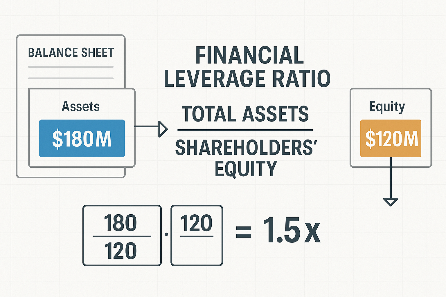
Financial Leverage Ratio = Average Total Assets ÷ Average Shareholders’ Equity
This ratio tells investors and analysts how many dollars of assets a company controls for every dollar of equity capital. A ratio of 2.0x means the company has $2 in total assets for every $1 of shareholder equity, indicating that half the asset base is financed through debt.
Why Averages Matter in Leverage Calculations
The formula uses average values rather than single-point measurements because balance sheets represent snapshots at specific dates. Averages smooth out seasonal fluctuations and provide a more representative picture of leverage throughout the period.
Average Total Assets = (Beginning Total Assets + Ending Total Assets) ÷ 2
Average Shareholders’ Equity = (Beginning Shareholders’ Equity + Ending Shareholders’ Equity) ÷ 2
This averaging methodology aligns with how analysts evaluate balance sheet basics and ensures that temporary spikes or dips don’t distort the leverage picture.
The Components That Drive the Formula
Total assets include everything a company owns: cash, inventory, equipment, real estate, intellectual property, and receivables. Understanding assets versus liabilities is fundamental to interpreting leverage correctly.
Shareholders’ equity represents the residual claim owners have after all liabilities are subtracted from assets. This includes:
- Common stock and preferred stock
- Additional paid-in capital
- Retained earnings (accumulated profits reinvested in the business)
- Treasury stock (if applicable)
The relationship between these components creates the mathematical foundation for understanding how debt amplifies business outcomes.
How the Financial Leverage Formula Works
The Financial Leverage Formula operates on a simple mathematical principle: when a company borrows money to acquire assets, it increases the denominator (total assets) without proportionally increasing the numerator (equity). This creates a multiplier effect on returns.
The Mechanics of Leverage Amplification
Consider a company with $100 million in equity that purchases $100 million in assets using only equity capital. The leverage ratio equals 1.0x ($100M ÷ $100M).
Now, suppose the same company instead uses its $100 million in equity as a foundation to borrow an additional $100 million. It now controls $200 million in assets with only $100 million in equity, creating a leverage ratio of 2.0x.
If those $200 million in assets generate a 10% return ($20 million), and the debt costs 5% annually ($5 million in interest), the company earns $15 million net. That $15 million return on $100 million equity equals 15%, significantly higher than the 10% it would have earned without leverage.
This amplification effect explains why companies pursue debt financing despite the risks. The math works in their favor as long as the return on assets exceeds the cost of debt.
The Double-Edged Sword Effect
Leverage amplifies losses with the same mathematical precision it amplifies gains. Using the same example, if the assets generate only a 3% return ($6 million) while debt still costs 5% ($5 million), the company nets only $1 million, a 1% return on equity instead of the 3% it would have earned without leverage.
If assets decline in value or generate negative returns, leverage accelerates the destruction of shareholder equity. This is why understanding the debt-to-equity ratio is critical for risk management.
Real-World Application Example
A practical example demonstrates how the Financial Leverage Formula works with actual numbers:
Company XYZ Financial Data:
- Beginning Total Assets (2024): $150 million
- Ending Total Assets (2025): $180 million
- Beginning Shareholders’ Equity (2024): $100 million
- Ending Shareholders’ Equity (2025): $120 million
Step 1: Calculate Average Total Assets
($150M + $180M) ÷ 2 = $165 million
Step 2: Calculate Average Shareholders’ Equity
($100M + $120M) ÷ 2 = $110 million
Step 3: Apply the Financial Leverage Formula
$165M ÷ $110M = 1.5x
This 1.5x ratio indicates that for every dollar of shareholder equity, the company controls $1.50 in total assets. The difference ($0.50 per equity dollar) represents debt financing.
The same company’s debt ratio would show that approximately 33% of assets are financed through debt ($55M debt ÷ $165M assets), while 67% comes from equity.
Degree of Financial Leverage (DFL): A Deeper Formula
While the basic Financial Leverage Formula measures the structural relationship between assets and equity, the Degree of Financial Leverage (DFL) quantifies how sensitive earnings per share are to changes in operating income.
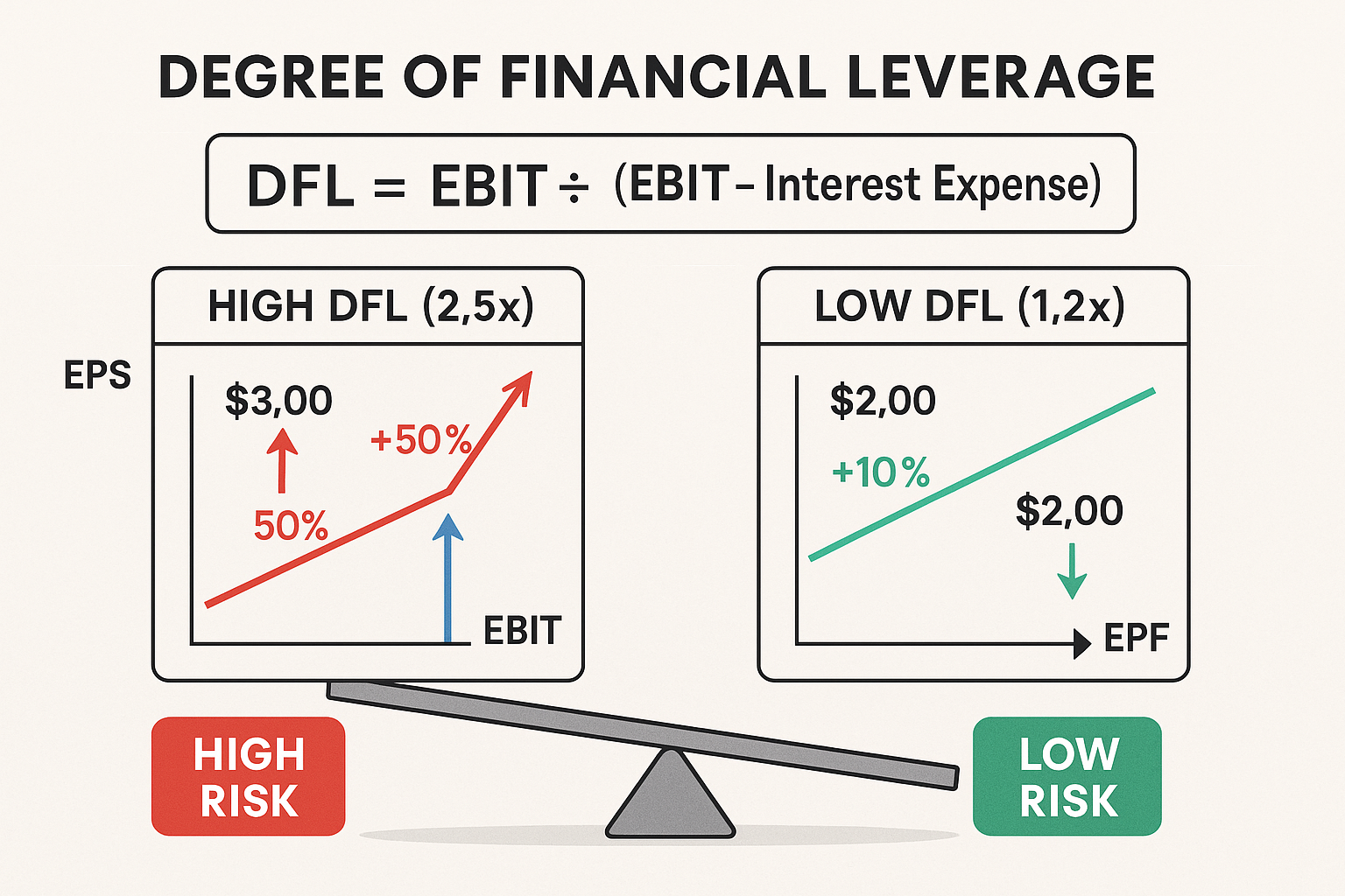
The DFL formula is:
DFL = EBIT ÷ (EBIT – Interest Expenses)
Where EBIT represents Earnings Before Interest and Taxes, essentially, operating profit before financing costs are deducted.
Understanding DFL Through Calculation
Consider a company with the following financials:
- EBIT: $500,000
- Interest Expenses: $100,000
DFL Calculation:
$500,000 ÷ ($500,000 – $100,000) = $500,000 ÷ $400,000 = 1.25
This 1.25 DFL means that a 1% change in EBIT results in a 1.25% change in earnings per share. The leverage amplifies operating performance fluctuations by 25%.
High DFL vs Low DFL: Risk Implications
High DFL (above 2.0) indicates significant financial risk. Small changes in operating income create large swings in earnings per share because interest expenses consume a substantial portion of operating profit.
For example, a company with a DFL of 3.0 would see a 10% increase in EBIT translate to a 30% increase in EPS, attractive during growth periods but devastating during downturns when a 10% EBIT decline causes a 30% EPS collapse.
Low DFL (below 1.5) reflects conservative financing with minimal debt. EPS fluctuations closely track operating income changes because interest expenses represent a small portion of EBIT.
This relationship between operating leverage and financial leverage is explored in depth through combined leverage analysis, which shows how both types of leverage interact to determine total business risk.
The DFL-to-Risk Translation
The mathematical relationship captured by DFL directly translates to investment risk. Higher DFL companies experience greater earnings volatility, which typically results in:
- More volatile stock prices
- Higher cost of equity capital (investors demand greater returns for increased risk)
- Greater bankruptcy risk during economic downturns
- Amplified returns during economic expansions
Understanding this cause-and-effect relationship enables investors to make data-driven decisions about whether a company’s leverage profile matches their risk tolerance and return objectives.
Alternative Financial Leverage Formulas
While the primary Financial Leverage Formula uses total assets and equity, several alternative formulas measure leverage from different analytical perspectives.
Debt-to-Assets Ratio
This formula measures what percentage of a company’s assets are financed through debt:
Debt-to-Assets Ratio = Total Debt ÷ Total Assets
A ratio of 0.40 means 40% of assets are debt-financed, while 60% are equity-financed. This provides a direct percentage view of leverage rather than a multiplier.
Debt-to-Equity Ratio
The debt-to-equity ratio compares borrowed capital directly to shareholder capital:
Debt-to-Equity Ratio = Total Debt ÷ Total Equity
A 1.0 ratio indicates equal amounts of debt and equity. A 2.0 ratio means the company has twice as much debt as equity—a more aggressive capital structure.
Equity Multiplier
The equity multiplier is mathematically equivalent to the Financial Leverage Formula, but emphasizes the multiplication effect:
Equity Multiplier = Total Assets ÷ Total Equity
This is the same calculation as the primary Financial Leverage Formula, but the name emphasizes how assets “multiply” the equity base through leverage.
Capitalization Ratio
The capitalization ratio focuses specifically on the long-term financing structure:
Capitalization Ratio = Long-Term Debt ÷ (Long-Term Debt + Shareholders’ Equity)
This formula excludes short-term debt to focus on permanent capital structure decisions, providing insight into strategic financing choices rather than working capital management.
Components of Financial Leverage: Assets and Equity Breakdown
Understanding what comprises the numerator and denominator in the Financial Leverage Formula is essential for accurate analysis and interpretation.
Total Assets: The Complete Picture
Total assets represent everything a company owns or controls that has economic value. These fall into two categories:
Current Assets (convertible to cash within one year):
- Cash and cash equivalents
- Marketable securities
- Accounts receivable
- Inventory
- Prepaid expenses
Non-Current Assets (long-term value):
- Property, plant, and equipment (PP&E)
- Intangible assets (patents, trademarks, goodwill)
- Long-term investments
- Deferred tax assets
The total of these components forms the numerator in the Financial Leverage Formula. Companies with asset-heavy business models (manufacturing, real estate) typically show higher absolute asset values than asset-light businesses (software, consulting).
Shareholders’ Equity: The Ownership Stake
Shareholders’ equity represents the residual value belonging to owners after all debts are paid. This includes:
Contributed Capital:
- Common stock (par value)
- Preferred stock
- Additional paid-in capital (amounts paid above par value)
Retained Earnings:
- Cumulative profits reinvested in the business
- Reduced by dividends paid to shareholders
- Can be negative if cumulative losses exceed profits
Other Comprehensive Income:
- Unrealized gains/losses on certain investments
- Foreign currency translation adjustments
- Pension liability adjustments
Understanding equity fundamentals helps investors interpret whether equity growth comes from profitable operations (retained earnings) or capital raises (contributed capital).
Debt Components in Leverage Analysis
While debt doesn’t appear explicitly in the basic Financial Leverage Formula, it’s the implicit difference between total assets and equity. Debt components include:
Short-Term Debt:
- Lines of credit
- Commercial paper
- Current portion of long-term debt
- Accounts payable
Long-Term Debt:
- Corporate bonds
- Term loans
- Mortgages
- Lease obligations
The composition and maturity profile of debt significantly affect financial risk beyond what the leverage ratio alone reveals. A company with a 2.0x leverage ratio faces very different risks if its debt matures in 30 days versus 30 years.
Financial Leverage Formula Examples: Step-by-Step Calculations
Working through detailed examples solidifies understanding of how the Financial Leverage Formula operates in practice.
Example 1: Moderate Leverage Manufacturing Company
ABC Manufacturing Balance Sheet Data:
January 1, 2025:
- Total Assets: $500 million
- Shareholders’ Equity: $300 million
- Total Debt: $200 million
December 31, 2025:
- Total Assets: $550 million
- Shareholders’ Equity: $330 million
- Total Debt: $220 million
Calculation:
Average Total Assets = ($500M + $550M) ÷ 2 = $525 million
Average Shareholders’ Equity = ($300M + $330M) ÷ 2 = $315 million
Financial Leverage Ratio = $525M ÷ $315M = 1.67x
Interpretation: ABC Manufacturing uses moderate leverage, with $1.67 in assets for every dollar of equity. Approximately 40% of assets are debt-financed [($525M – $315M) ÷ $525M], indicating a balanced capital structure suitable for a stable manufacturing operation.
Example 2: High Leverage Real Estate Investment Trust
XYZ REIT Balance Sheet Data:
Q1 2025:
- Total Assets: $2 billion
- Shareholders’ Equity: $600 million
- Total Debt: $1.4 billion
Q4 2025:
- Total Assets: $2.2 billion
- Shareholders’ Equity: $650 million
- Total Debt: $1.55 billion
Calculation:
Average Total Assets = ($2.0B + $2.2B) ÷ 2 = $2.1 billion
Average Shareholders’ Equity = ($600M + $650M) ÷ 2 = $625 million
Financial Leverage Ratio = $2.1B ÷ $625M = 3.36x
Interpretation: XYZ REIT employs aggressive leverage typical of real estate investment trusts. With $3.36 in assets per equity dollar, approximately 70% of assets are debt-financed. This high leverage is common in REIT investing because stable rental income supports debt service, but it also creates significant interest rate risk.
Example 3: Low Leverage Technology Company
Tech Innovators Inc. Balance Sheet Data:
Beginning of Year:
- Total Assets: $800 million
- Shareholders’ Equity: $700 million
- Total Debt: $100 million
End of Year:
- Total Assets: $900 million
- Shareholders’ Equity: $800 million
- Total Debt: $100 million
Calculation:
Average Total Assets = ($800M + $900M) ÷ 2 = $850 million
Average Shareholders’ Equity = ($700M + $800M) ÷ 2 = $750 million
Financial Leverage Ratio = $850M ÷ $750M = 1.13x
Interpretation: Tech Innovators maintains minimal leverage, with only $0.13 of debt per equity dollar. Approximately 12% of assets are debt-financed, indicating a conservative capital structure. This is common among profitable technology companies that generate sufficient cash flow to fund growth without significant borrowing.
Example 4: Degree of Financial Leverage Calculation
Company DFL Analysis:
Operating Data:
- EBIT: $800,000
- Interest Expenses: $150,000
- Shares Outstanding: 100,000
DFL Calculation:
DFL = $800,000 ÷ ($800,000 – $150,000) = $800,000 ÷ $650,000 = 1.23
Scenario Analysis:
If EBIT increases by 10% to $880,000:
- New EBT (Earnings Before Tax) = $880,000 – $150,000 = $730,000
- Percentage increase in EBT = ($730,000 – $650,000) ÷ $650,000 = 12.3%
The DFL of 1.23 correctly predicts that a 10% EBIT increase produces a 12.3% increase in pre-tax earnings (10% × 1.23 = 12.3%).
This mathematical relationship demonstrates how the degree of operating leverage and financial leverage combine to determine total earnings sensitivity.
When Financial Leverage Works (and When It Doesn’t)
The Financial Leverage Formula reveals the structure of leverage, but understanding when leverage creates value versus destroys it requires examining the relationship between returns and costs.
The Fundamental Leverage Equation
Leverage creates value when:
Return on Assets (ROA) > Cost of Debt
If a company can earn 12% on assets while paying 6% on debt, the 6% spread accrues entirely to equity holders, amplifying returns.
Leverage destroys value when:
Return on Assets (ROA) < Cost of Debt
If assets earn only 4% while debt costs 6%, the company loses 2% on every borrowed dollar, reducing shareholder returns below what they would be without leverage.
Industry-Specific Leverage Norms
Different industries operate with vastly different leverage profiles based on asset stability, cash flow predictability, and growth requirements:
High Leverage Industries (2.5x – 4.0x):
- Utilities (stable, regulated cash flows)
- Real estate (tangible collateral, predictable rents)
- Telecommunications (infrastructure-heavy, recurring revenue)
Moderate Leverage Industries (1.5x – 2.5x):
- Manufacturing (cyclical but asset-backed)
- Retail (inventory and real estate collateral)
- Transportation (equipment-intensive)
Low Leverage Industries (1.0x – 1.5x):
- Technology (intangible assets, rapid change)
- Biotechnology (high R&D risk, uncertain outcomes)
- Professional services (minimal asset requirements)
Comparing a company’s Financial Leverage Ratio to industry norms provides context for whether its capital structure is appropriate or excessive.
The Leverage-Growth Relationship
Companies in high-growth phases often use leverage strategically to accelerate expansion. The math works because:
- Growth investments generate returns that exceed debt costs
- Future cash flows justify current borrowing
- Market share gains create competitive advantages worth the financial risk
However, this strategy requires precise execution. Growth must materialize as projected, or the debt burden becomes unsustainable.
Conservative investors often prefer companies that fund growth through retained earnings rather than debt, accepting slower expansion in exchange for lower risk—a philosophy aligned with dividend reinvestment strategies.
Economic Cycle Considerations
Leverage performance varies dramatically across economic cycles:
Expansion Phases:
- Rising revenues cover interest expenses easily
- Asset values appreciate, improving debt-to-asset ratios
- Access to refinancing improves, reducing debt costs
Recession Phases:
- Declining revenues strain debt service capacity
- Asset values fall, worsening leverage ratios
- Credit markets tighten, increasing borrowing costs or eliminating access entirely
The 2008 financial crisis demonstrated how excessive leverage destroys companies during downturns, even when the underlying business model is sound. Companies with Financial Leverage Ratios above 3.0x faced severe distress, while those below 2.0x weathered the storm more successfully.
Financial Leverage and Risk Management
Understanding the Financial Leverage Formula enables proactive risk management through quantitative analysis and strategic decision-making.
Leverage Limits and Covenants
Lenders impose leverage limits through debt covenants that restrict how much a company can borrow relative to equity or earnings. Common covenant structures include:
Maximum Debt-to-Equity Ratio: Prevents leverage from exceeding specified levels (e.g., 2.5x)
Minimum Interest Coverage Ratio: Requires EBIT to exceed interest expenses by a specified multiple (e.g., 3.0x)
Maximum Debt-to-EBITDA Ratio: Limits total debt relative to cash generation capacity
Violating these covenants triggers technical default, potentially accelerating debt repayment or increasing interest rates. Monitoring the Financial Leverage Formula helps companies maintain covenant compliance.
Deleveraging Strategies
When leverage becomes excessive, companies employ deleveraging strategies to reduce risk:
Asset Sales: Selling non-core assets generates cash to repay debt, reducing both the numerator (assets) and the implicit debt component
Equity Issuance: Raising capital through stock sales increases the denominator (equity) while using proceeds to reduce debt
Earnings Retention: Suspending dividends and retaining all profits gradually builds equity, reducing the leverage ratio over time
Debt Restructuring: Negotiating with creditors to convert debt to equity or extend maturities
Each strategy involves trade-offs. Asset sales may sacrifice future earnings potential. Equity issuance dilutes existing shareholders. Dividend suspension disappoints income investors. The optimal approach depends on the specific situation and market conditions.
Leverage and Valuation Impact
The Financial Leverage Formula directly affects company valuation through multiple channels:
Cost of Capital: Higher leverage increases financial risk, raising the cost of equity capital that investors demand. This higher discount rate reduces the present value of future cash flows.
Earnings Volatility: Greater DFL creates more volatile earnings, which markets typically value at lower multiples due to increased uncertainty.
Bankruptcy Risk: Excessive leverage increases the probability of financial distress, reducing enterprise value through expected bankruptcy costs.
Tax Benefits: Debt interest is tax-deductible, creating a “tax shield” that increases after-tax cash flows and company value (within reasonable leverage limits).
The optimal capital structure balances these competing effects, maximizing value by using enough leverage to capture tax benefits without creating excessive financial risk.
Comparing Financial Leverage Across Companies
The Financial Leverage Formula becomes most powerful when used for comparative analysis across companies, industries, and time periods.
Peer Group Comparison Framework
Effective leverage comparison requires selecting appropriate peer companies:
- Same Industry: Compare retailers to retailers, not retailers to software companies
- Similar Size: Large-cap companies access capital differently than small-caps
- Comparable Business Models: Asset-light vs. asset-heavy models justify different leverage levels
- Geographic Similarity: Regulatory environments and credit markets vary by region
Interpreting Leverage Differences
When Company A shows a 2.5x Financial Leverage Ratio while Company B shows 1.5x, several explanations may apply:
Strategic Choice: Company A pursues aggressive growth through debt financing, while Company B prefers conservative organic growth
Life Cycle Stage: Mature companies with stable cash flows can support higher leverage than early-stage companies with uncertain revenues
Asset Composition: Companies with tangible, liquid assets (real estate, equipment) can sustain higher leverage than those with intangible assets (intellectual property, goodwill)
Management Philosophy: Some management teams prioritize financial flexibility over return maximization, maintaining lower leverage intentionally
Understanding these contextual factors prevents misinterpretation of leverage ratios in isolation.
Time-Series Leverage Analysis
Tracking a single company’s Financial Leverage Ratio over time reveals strategic shifts and financial trends:
Rising Leverage Trends may indicate:
- Debt-funded acquisitions or expansion
- Declining profitability, reducing equity through losses
- Strategic shift toward a more aggressive capital structure
- Deteriorating financial health requires investigation
Declining Leverage Trends may indicate:
- Deleveraging after a period of high borrowing
- Strong profitability is building retained earnings
- Asset sales are reducing the asset base
- Equity raises diluting existing shareholders
Combining leverage analysis with profitability metrics like EBITDA and economic profit provides comprehensive insight into financial performance and strategy.
Financial Leverage Formula in Investment Decision-Making
Investors use the Financial Leverage Formula to assess risk, predict returns, and construct portfolios aligned with their objectives.
Leverage and Expected Returns
The mathematical relationship between leverage and returns follows a predictable pattern:
Expected Return on Equity = ROA + (ROA – Cost of Debt) × Debt-to-Equity Ratio
This formula shows how leverage amplifies the spread between asset returns and debt costs. When ROA exceeds debt costs, higher leverage increases equity returns. When ROA falls below debt costs, leverage accelerates losses.
Sophisticated investors calculate expected returns under various scenarios, weighting them by probability to determine whether a company’s leverage profile offers attractive risk-adjusted returns.
Leverage Screening Criteria
Many investment strategies incorporate leverage thresholds as screening criteria:
Conservative Value Investing:
- Maximum Financial Leverage Ratio: 2.0x
- Maximum Debt-to-Equity: 1.0x
- Minimum Interest Coverage: 5.0x
Dividend Income Investing:
- Maximum Financial Leverage Ratio: 2.5x
- Focus on stable, predictable leverage
- Preference for declining leverage trends
Growth Investing:
- More flexible leverage tolerance
- Emphasis on whether debt funds are productive growth
- Analysis of leverage sustainability as growth matures
These criteria help investors systematically identify companies whose leverage profiles match their risk tolerance and investment philosophy, similar to how the 50/30/20 rule provides structure for personal budgeting decisions.
Portfolio-Level Leverage Considerations
Beyond individual stock analysis, investors consider aggregate portfolio leverage:
Diversification Benefits: Holding multiple companies with different leverage profiles reduces concentration risk from any single company’s capital structure
Sector Allocation: Overweighting low-leverage sectors (technology) versus high-leverage sectors (utilities) affects overall portfolio risk
Economic Sensitivity: High-leverage portfolios amplify both gains and losses during economic cycles, requiring appropriate risk management
Correlation Effects: Leverage-related risks often correlate during financial crises, reducing diversification benefits when they’re needed most
Understanding these portfolio-level dynamics helps investors construct allocations that deliver desired risk-return profiles across market environments.
Advanced Applications of the Financial Leverage Formula
Beyond basic leverage measurement, sophisticated analysts use the Financial Leverage Formula in complex analytical frameworks.
DuPont Analysis Integration
The Financial Leverage Formula forms one component of the DuPont identity, which decomposes return on equity into three drivers:
ROE = Net Profit Margin × Asset Turnover × Financial Leverage
Or more specifically:
ROE = (Net Income ÷ Sales) × (Sales ÷ Assets) × (Assets ÷ Equity)
This framework reveals whether ROE comes from operational efficiency (margin), asset productivity (turnover), or leverage. Two companies with identical 15% ROE may achieve it through entirely different means:
- Company A: 5% margin × 1.5 turnover × 2.0 leverage = 15% ROE
- Company B: 10% margin × 1.0 turnover × 1.5 leverage = 15% ROE
Company A relies more heavily on leverage to achieve its returns, while Company B achieves similar results through superior profitability. This distinction matters for sustainability and risk assessment.
Combined Leverage Analysis
Combined leverage multiplies operating leverage by financial leverage to measure total earnings volatility:
Degree of Combined Leverage (DCL) = DOL × DFL
Where:
- DOL = Degree of Operating Leverage (sensitivity of EBIT to sales changes)
- DFL = Degree of Financial Leverage (sensitivity of EPS to EBIT changes)
A company with a DOL of 2.0 and a DFL of 1.5 has a DCL of 3.0, meaning a 1% sales change produces a 3% EPS change. This amplification occurs through two stages: sales changes affect EBIT (operating leverage), then EBIT changes affect EPS (financial leverage).
Understanding combined leverage helps investors predict earnings volatility under various revenue scenarios.
Leverage in Credit Analysis
Credit analysts use the Financial Leverage Formula alongside other metrics to assess default risk:
Credit Rating Factors:
- Leverage ratios (multiple formulations)
- Interest coverage ratios
- Cash flow adequacy
- Asset quality and liquidity
- Industry position and competitive dynamics
The Altman Z-Score incorporates leverage as one of five factors predicting bankruptcy probability, demonstrating how leverage interacts with other financial metrics to determine credit risk.
Companies approaching financial distress typically show:
- Rising Financial Leverage Ratios
- Declining interest coverage
- Negative or minimal retained earnings growth
- Asset sales to service debt
- Deteriorating working capital positions
Recognizing these patterns early enables investors to avoid losses or negotiate better terms as creditors.
Common Mistakes in Financial Leverage Analysis
Even experienced analysts make errors when calculating or interpreting the Financial Leverage Formula. Avoiding these pitfalls improves analytical accuracy.
Mistake 1: Using Point-in-Time Values Instead of Averages
Calculating leverage using only year-end balance sheet values misses intra-period fluctuations. A company that acquires another business on December 30 shows dramatically different leverage than one day earlier, but the single-day difference doesn’t represent typical leverage throughout the year.
Solution: Always use average values calculated from beginning and ending period balances, or ideally, quarterly averages for more precision.
Mistake 2: Ignoring Off-Balance-Sheet Obligations
Traditional balance sheets may not capture all leverage-creating obligations:
- Operating leases (though improved under current accounting standards)
- Pension obligations
- Contingent liabilities
- Joint venture debt
- Special-purpose entity obligations
Solution: Adjust leverage calculations to include material off-balance-sheet items, particularly when comparing companies across different accounting regimes or time periods.
Mistake 3: Comparing Leverage Across Incompatible Industries
A 3.0x Financial Leverage Ratio represents conservative financing for a utility company but aggressive leverage for a software company. Industry economics determine appropriate leverage levels.
Solution: Always compare leverage ratios to industry-specific benchmarks and understand the business model characteristics that justify different leverage levels.
Mistake 4: Overlooking Leverage Quality Differences
Two companies with identical 2.0x Financial Leverage Ratios face different risks if one has fixed-rate 30-year debt while the other has variable-rate debt maturing in six months.
Solution: Examine debt composition, maturity schedule, interest rate structure, and covenant restrictions alongside headline leverage ratios.
Mistake 5: Failing to Adjust for Goodwill and Intangibles
Goodwill and intangible assets inflate total assets but provide minimal value in financial distress. A company with $100 million in equity and $200 million in assets appears to have 2.0x leverage, but if $80 million of assets are goodwill, the tangible leverage is much higher.
Solution: Calculate tangible leverage ratios that exclude goodwill and intangibles for a more conservative risk assessment, particularly in asset-heavy industries or post-acquisition scenarios.
Financial Leverage Formula: Practical Implementation Guide
Implementing leverage analysis in real-world investment or business decision-making requires systematic processes and disciplined interpretation.
Step-by-Step Leverage Analysis Process
Step 1: Gather Balance Sheet Data
- Obtain beginning and ending period balance sheets
- Verify data accuracy and consistency
- Identify any accounting changes or restatements
Step 2: Calculate Component Averages
- Average total assets
- Average shareholders’ equity
- Average debt (if calculating debt-specific ratios)
Step 3: Compute Primary Leverage Metrics
- Financial Leverage Ratio (Assets ÷ Equity)
- Debt-to-Equity Ratio
- Debt-to-Assets Ratio
Step 4: Calculate Degree of Financial Leverage
- Obtain EBIT from the income statement
- Identify total interest expenses
- Apply the DFL formula
Step 5: Perform Comparative Analysis
- Compare to historical company trends
- Benchmark against industry peers
- Assess relative to credit rating standards
Step 6: Conduct Scenario Analysis
- Model leverage under revenue growth scenarios
- Test sensitivity to interest rate changes
- Evaluate covenant compliance margins
Step 7: Synthesize Findings and Make Decisions
- Integrate leverage analysis with broader financial assessment
- Determine whether the leverage profile aligns with the investment criteria
- Identify specific risks requiring monitoring
Building a Leverage Monitoring Dashboard
Systematic leverage monitoring prevents surprises and enables proactive management:
Quarterly Metrics to Track:
- Financial Leverage Ratio (trend over 8+ quarters)
- Debt-to-Equity Ratio
- Interest Coverage Ratio
- Debt maturity schedule
- Covenant compliance status
Annual Deep-Dive Analysis:
- Peer group leverage comparison
- Capital structure optimization assessment
- Debt refinancing opportunities
- Strategic leverage targets
Trigger Points for Action:
- Leverage ratio exceeding industry average by >20%
- Interest coverage falling below 3.0x
- Approaching covenant violation (within 10% of limit)
- Credit rating downgrade or negative outlook
- Significant adverse change in business fundamentals
This systematic approach transforms the Financial Leverage Formula from an academic concept into a practical risk management tool.
📊 Financial Leverage Calculator
Calculate your company’s leverage ratio and degree of financial leverage
Balance Sheet Data
Income Statement Data (Optional – for DFL)
The Relationship Between Financial Leverage and Other Financial Metrics
The Financial Leverage Formula doesn’t exist in isolation—it interacts with numerous other financial metrics to create a comprehensive picture of company performance and risk.
Leverage and Return on Equity (ROE)
Financial leverage directly amplifies ROE through the mathematical relationship:
ROE = ROA × Financial Leverage Ratio (simplified form)
More precisely:
ROE = ROA + (ROA – Cost of Debt) × (Debt ÷ Equity)
This formula demonstrates that leverage increases ROE when ROA exceeds the cost of debt. The higher the leverage ratio, the greater the amplification, for better or worse.
A company with 10% return on assets(ROA) and 6% debt cost can dramatically increase return on equity (ROE) by adding leverage:
- At 1.0x leverage (no debt): ROE = 10%
- At 2.0x leverage: ROE ≈ 14%
- At 3.0x leverage: ROE ≈ 18%
However, if ROA falls to 4% while debt costs remain at 6%, leverage destroys value:
- At 1.0x leverage: ROE = 4%
- At 2.0x leverage: ROE ≈ 2%
- At 3.0x leverage: ROE ≈ 0%
Leverage and Liquidity Ratios
Financial leverage affects liquidity metrics like the current ratio and cash ratio because debt creates payment obligations that consume liquid assets.
High leverage typically correlates with:
- Lower current ratios (debt payments reduce working capital)
- Tighter cash positions (interest and principal payments drain cash)
- Greater reliance on refinancing (maturing debt must be rolled over)
Companies with leverage ratios above 3.0x often show current ratios below 1.5x, indicating potential liquidity stress during downturns.
Leverage and Profitability Metrics
The interaction between leverage and profitability determines whether debt creates or destroys value:
EBITDA Margin: Higher margins provide a greater cushion to cover interest expenses, making leverage more sustainable
Earnings Per Share: Leverage amplifies EPS growth during expansions but accelerates EPS declines during contractions
Economic Profit: True economic profit accounts for the cost of both debt and equity capital, revealing whether leverage actually creates value after all capital costs
Leverage and Valuation Multiples
Market valuation multiples reflect leverage levels because investors price in financial risk:
Price-to-Book Ratio: High leverage reduces book value relative to market value, often resulting in higher P/B multiples for leveraged companies
Enterprise Value-to-EBITDA: This metric neutralizes capital structure differences by adding debt back to market capitalization, enabling comparison across different leverage profiles
Price-to-Earnings Ratio: Leverage increases earnings volatility, which markets typically discount through lower P/E multiples for highly leveraged companies
Understanding these relationships enables investors to determine whether a company’s valuation appropriately reflects its leverage-related risks.
Financial Leverage in Personal Finance Applications
While the Financial Leverage Formula primarily applies to corporate analysis, the underlying principles extend to personal financial decisions.
Mortgage Leverage
Homeownership represents the most common form of personal financial leverage. A homebuyer with $100,000 down payment who purchases a $500,000 home creates a personal leverage ratio of 5.0x ($500,000 ÷ $100,000).
The mathematics work identically to corporate leverage:
- If the home appreciates 10% ($50,000), the owner’s equity increases 50% ($50,000 ÷ $100,000)
- If the home depreciates 10% ($50,000), the owner’s equity decreases 50%
The 3x rent rule and 20/4/10 rule for car buying represent practical applications of leverage principles to consumer decisions, ensuring debt obligations remain sustainable relative to income.
Investment Account Leverage
Margin investing allows individuals to borrow against portfolio holdings to purchase additional securities, creating investment leverage. A $100,000 portfolio with 50% margin ($50,000 borrowed) creates 2.0x leverage.
The risks mirror corporate leverage:
- Returns amplify when investments perform well
- Losses accelerate when investments decline
- Margin calls force liquidation during market downturns
- Interest costs reduce net returns
Conservative investors typically avoid margin leverage entirely, preferring the stability of unleveraged positions aligned with evidence-based investing principles.
Student Loan Leverage
Education financing represents leverage on future earning capacity. A student borrowing $100,000 for education that increases lifetime earnings by $500,000 creates positive leverage—the return on the “asset” (enhanced earning capacity) exceeds the cost of debt.
However, if education doesn’t increase earnings sufficiently to justify the debt cost, leverage destroys value. This calculation requires an honest assessment of expected returns versus debt obligations.
Personal Leverage Limits
Unlike corporations with sophisticated treasury departments, individuals face greater consequences from excessive leverage:
- Limited refinancing options during financial distress
- Personal bankruptcy affects creditworthiness for years
- Psychological stress from debt burden impairs decision-making
- Reduced financial flexibility limits career and life choices
Prudent personal leverage typically stays well below corporate norms, with total debt-to-asset ratios below 50% and debt service consuming less than 30% of income.
Conclusion: Mastering the Financial Leverage Formula for Smarter Decisions
The Financial Leverage Formula transforms abstract balance sheet data into actionable intelligence about risk, return potential, and financial sustainability. By quantifying the precise relationship between assets, equity, and debt, this formula enables data-driven decisions for investors, business managers, and financial analysts.
Understanding that leverage acts as a mathematical amplifier—magnifying both gains and losses with predictable precision—fundamentally changes how informed investors evaluate companies and opportunities. A 2.0x leverage ratio isn’t just a number; it represents a specific, calculable relationship between borrowed capital and ownership capital that determines how business performance translates to shareholder returns.
The Degree of Financial Leverage extends this analysis by revealing how operating income fluctuations affect earnings per share, providing quantitative insight into earnings volatility and financial risk. A DFL of 2.5 tells investors that earnings will swing 2.5% for every 1% change in operating profit—critical information for risk assessment and portfolio construction.
Actionable Next Steps
For Investors:
- Calculate the Financial Leverage Ratio for all portfolio holdings using the formula: Average Total Assets ÷ Average Shareholders’ Equity
- Compare company leverage ratios to industry benchmarks to identify outliers requiring additional analysis
- Monitor leverage trends over time, investigating significant increases or decreases
- Incorporate leverage analysis into investment screening criteria aligned with your risk tolerance
- Assess whether current valuations appropriately reflect leverage-related risks
For Business Managers:
- Track your company’s Financial Leverage Ratio quarterly to monitor capital structure evolution
- Calculate DFL to understand how operating performance fluctuations affect earnings per share
- Model leverage under various growth scenarios to determine optimal capital structure
- Establish leverage targets and covenant buffers to maintain financial flexibility
- Consider deleveraging strategies if ratios exceed industry norms or create refinancing risk
For Financial Learners:
- Practice calculating leverage ratios using real company financial statements from public filings
- Build a comparison spreadsheet tracking leverage across multiple companies in an industry
- Study how leverage ratios changed during the 2008 financial crisis and the 2020 pandemic
- Explore the relationship between leverage and stock price volatility in your portfolio
- Integrate leverage analysis with other financial metrics for a comprehensive company evaluation
The math behind money becomes clear when leverage formulas transform balance sheet abstractions into concrete risk-return relationships. Companies that master an optimal leverage balance grow with financial stability. Investors who understand leverage mathematics avoid value traps while identifying opportunities others miss.
Financial leverage represents neither inherent good nor evil—it’s a tool whose outcomes depend entirely on the mathematical relationship between returns earned and costs paid. By mastering the Financial Leverage Formula and its applications, you gain the analytical foundation to evaluate this critical relationship with precision and confidence.
The numbers tell the story. The formula reveals the truth. Your decisions determine the outcome.
References
[1] Corporate Finance Institute – Financial Leverage Ratio Analysis (www.corporatefinanceinstitute.com)
[2] CFA Institute – Capital Structure and Leverage (www.cfainstitute.org)
[3] Federal Reserve Economic Data – Corporate Debt Statistics (fred.stlouisfed.org)
[4] Securities and Exchange Commission – Financial Statement Analysis Guide (www.sec.gov)
[5] Investopedia – Degree of Financial Leverage (www.investopedia.com)
[6] Morningstar – Leverage Ratio Benchmarks by Industry (www.morningstar.com)
[7] Financial Accounting Standards Board – Balance Sheet Classification Standards (www.fasb.org)
Author Bio
Max Fonji is the founder of The Rich Guy Math, a data-driven financial education platform dedicated to explaining the mathematical principles behind wealth building, investing, and risk management. With a background in financial analysis and a commitment to evidence-based investing, Max translates complex financial concepts into clear, actionable insights for investors at all levels. His work emphasizes understanding cause-and-effect relationships in finance through quantitative analysis and rational decision-making frameworks.
Educational Disclaimer
This article is provided for educational and informational purposes only and does not constitute financial, investment, tax, or legal advice. The Financial Leverage Formula and related concepts are analytical tools that should be used as part of comprehensive financial analysis, not as sole decision-making criteria.
Financial leverage involves significant risks, including the potential for amplified losses and financial distress. Past performance and historical leverage ratios do not guarantee future results. Individual companies, industries, and economic conditions vary substantially, requiring context-specific analysis.
Readers should conduct their own due diligence and consult with qualified financial advisors, accountants, and legal professionals before making investment decisions or implementing leverage strategies. The author and The Rich Guy Math assume no liability for financial decisions made based on this content.
All financial data, formulas, and examples presented are for illustrative purposes. Actual investment results may differ materially from examples provided. Always verify financial data from authoritative sources and understand the specific risks associated with leveraged investments or business operations.
Frequently Asked Questions
What is the Financial Leverage Formula?
The Financial Leverage Formula calculates the ratio between a company’s total assets and shareholders’ equity: Financial Leverage Ratio = Average Total Assets ÷ Average Shareholders’ Equity. This ratio measures how much debt a company uses relative to equity financing, with higher ratios indicating greater reliance on borrowed capital.
How do you calculate the Degree of Financial Leverage (DFL)?
The Degree of Financial Leverage is calculated as: DFL = EBIT ÷ (EBIT – Interest Expenses). This formula measures how sensitive earnings per share are to changes in operating income, with higher DFL values indicating greater earnings volatility from leverage.
What is a good Financial Leverage Ratio?
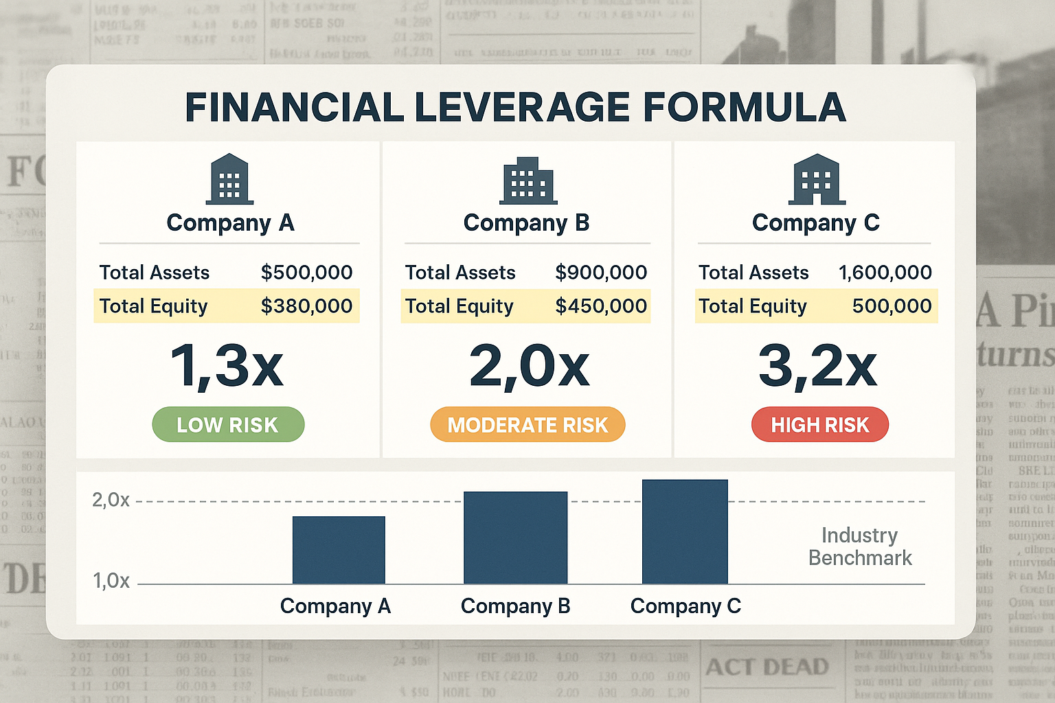
Appropriate leverage ratios vary by industry, but general guidelines suggest: below 1.5x indicates conservative leverage, 1.5x–2.5x represents moderate leverage typical of many industries, and above 3.0x indicates aggressive leverage requiring careful monitoring. Industry-specific benchmarks provide more accurate assessment standards.
What’s the difference between financial leverage and operating leverage?
Financial leverage measures how debt financing amplifies returns on equity, calculated from balance sheet relationships between assets and equity. Operating leverage measures how fixed costs amplify operating profit changes from revenue fluctuations, calculated from income statement cost structures. Combined leverage multiplies both effects to show total earnings sensitivity.
How does financial leverage affect return on equity?
Financial leverage amplifies ROE through the relationship: ROE = ROA + (ROA – Cost of Debt) × (Debt ÷ Equity). When return on assets exceeds debt costs, leverage increases ROE. When ROA falls below debt costs, leverage reduces ROE. The leverage ratio determines the magnitude of this amplification effect.
Can financial leverage be negative?
Financial leverage ratios are typically positive because both assets and equity are positive values. However, if shareholders’ equity becomes negative (accumulated losses exceed contributed capital), the leverage ratio becomes negative or undefined, indicating severe financial distress requiring immediate attention.
How often should companies calculate their Financial Leverage Ratio?
Companies should calculate leverage ratios quarterly at minimum, using average values from beginning and ending balance sheets. Monthly calculations provide better trend visibility for companies with volatile operations or those actively managing capital structure. Annual calculations are insufficient for timely risk management.
What’s the relationship between the Financial Leverage Formula and debt-to-equity ratio?
The Financial Leverage Formula (Assets ÷ Equity) and debt-to-equity ratio (Debt ÷ Equity) measure related but distinct concepts. Financial leverage shows total asset control per equity dollar, while debt-to-equity directly compares borrowed capital to ownership capital. The relationship is: Financial Leverage = 1 + Debt-to-Equity Ratio.